CS180-Computer Vision Finalterm Review & Cheatsheet

 2024/12/04 

Finalterm Review & Cheatsheet for
CS 180 Fall 2024 | Intro to Computer Vision and Computational Photography

Author: SimonXie2004.github.io

Resources

Download Cheatsheet (pdf)

Download Cheatsheet (pptx)

Download Cheatsheet (markdown+images)

Lec2 Capturing Light

Psychophysics of Color: Mean => Hue, Variance => Saturation, Area => Brightness
Image Processing Sequence
1. Auto Exposure -> White Balance -> Contrast -> Gamma
White Balancing Algorithms
1. Grey World: force average color of scene to grey
2. White World: force brightest object to white
Quad Bayer Filters
1. Why more green pixels? Because human are most sensitive to green light.
Color Spaces: RGB, CMY(K), HSV, L*a*b* (Perceptually uniform color space)
Image similarity:
1. SSD, i.e. L2 Distance
2. NCC, invariant to local avg and contrast
\[ \text{NCC}(I, T) = \frac{\sum_{x,y} (I'(x,y) \cdot T'(x,y))}{\sqrt{\sum_{x,y} I'(x,y)^2 \sum_{x,y} T'(x,y)^2}} \]

Lec 3-4: Pixels and Images

Lambertian Reflectance Model:
1. $(1-\rho)$ absorbed, $\rho$ reflected (either diffusely or specularly)
2. Diffuse Reflectance: $I(x) = \rho(x) \cdot \mathbf{S} \cdot \mathbf{N}(x)$
Image Acquisition Pipeline:
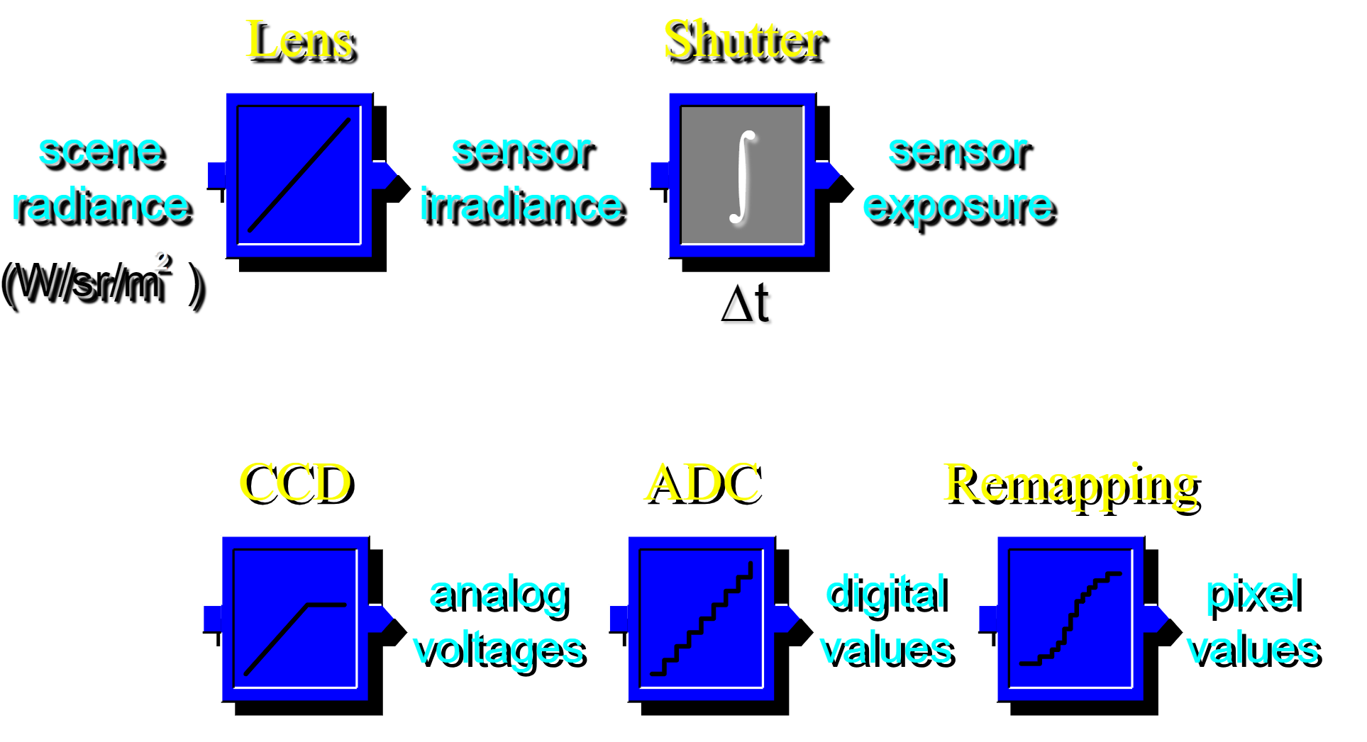
Image Processing: Gamma Correction
1. Power-law transformations: $s = c\cdot r^\gamma$
2. Contrast Stretching: S curve (from input gray level to output)
Histograms Matching and Color Transfer
Image Filter
1. Cross Correlation $C = K \times I$ or $C(u, v) = \sum_{x=0}^{M-1} \sum_{y=0}^{N-1} I(x, y) \cdot K(x+u, y+v)$
2. Convolution: $C = K * I$ or $C(u, v) = \sum_{x=0}^{M-1} \sum_{y=0}^{N-1} I(x, y) \cdot K(x-u, y-v)$
Example: Gaussian Filter
1. Rule of Thumb: Half-Width = $3\sigma$
Image Sub-sampling: Must first filter the image, then subsample (Anti-Aliasing)
Image Derivatives: To avoid the effects of noise, first smooth, then derivative (i.e. look for peaks in $\frac{d}{dx}(f*g)$)
1. This leads to LoG or DoG filters

Lec 5: Furrier Transform

Math:
1. Furrier Transform: $F(\omega) = \int_{-\infty}^{\infty} f(t) e^{-i \omega t} \, dt$
2. Inverse Transform: $f(t) = \frac{1}{2\pi} \int_{-\infty}^{\infty} F(\omega) e^{i \omega t} \, d\omega$
Low pass, High pass, Band pass filters
1. Details = High-freq components;
2. Sharpening Details: $f + \alpha (f - f * g) = (1+\alpha)f-af*g = f*((1+\alpha)e-\alpha g)$
3. Remark that $(1+\alpha)e-\alpha g$ is approximately Laplacian of Gaussian.

Lec 6: Pyramids Blending

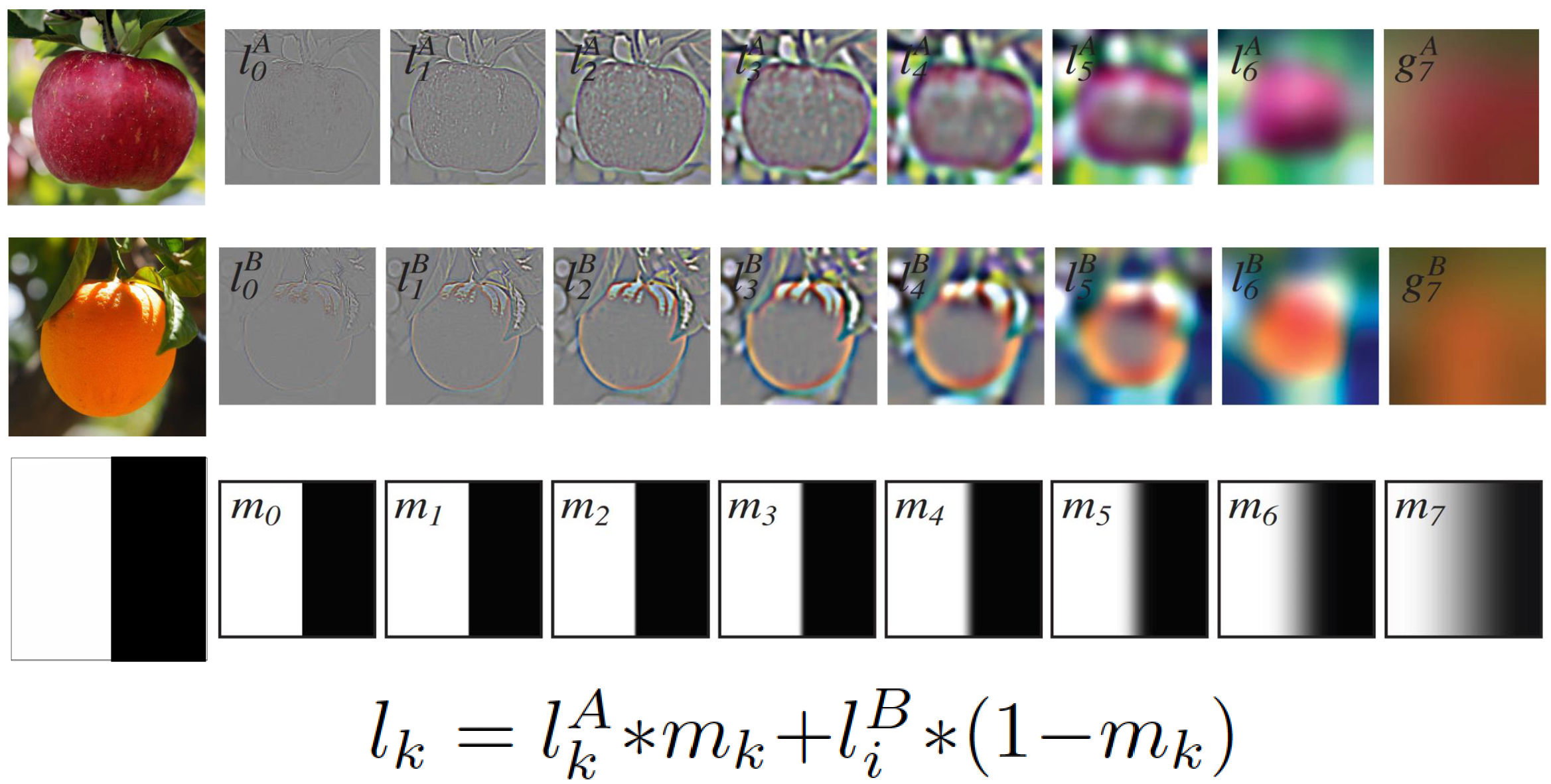
Gaussian Pyramids and Laplacian Pyramids (Remember to add lowest freq!)
Laplacian Pyramids and Image Blending:
Other image algorithms:
1. Denoising: Median Filter
2. Lossless Compression (PNG): Huffman Coding
3. Lossy Compression (JPEG): Block-based Discrete Cosine Transform (DCT)
  1. Compute DCT Coefficients; Coarsely Quantize; Encode (e.g. with Huffman Coding)

Lec 7-9 Affine Transformations

Transform Matrices
1. Scaling, Shearing and Translation: $S = \begin{bmatrix} a & sh_x & t_x \\ sh_y & b & t_y \\ 0 & 0 & 1\end{bmatrix}$
2. Rotation: $R = \begin{bmatrix} \cos(\theta) & -\sin(\theta) & 0\\ \sin(\theta) & \cos(\theta) & 0 \\ 0 & 0 & 1 \end{bmatrix}$
Calculating Affine Matrix: \[ \begin{pmatrix} a & b & tx \\ c & d & ty \\ 0 & 0 & 1 \end{pmatrix} \cdot \begin{pmatrix} x_1 & x_2 & x_3 \\ y_1 & y_2 & y_3 \\ 1 & 1 & 1 \end{pmatrix} = \begin{pmatrix} x_1' & x_2' & x_3' \\ y_1' & y_2' & y_3' \\ 1 & 1 & 1 \end{pmatrix} \]
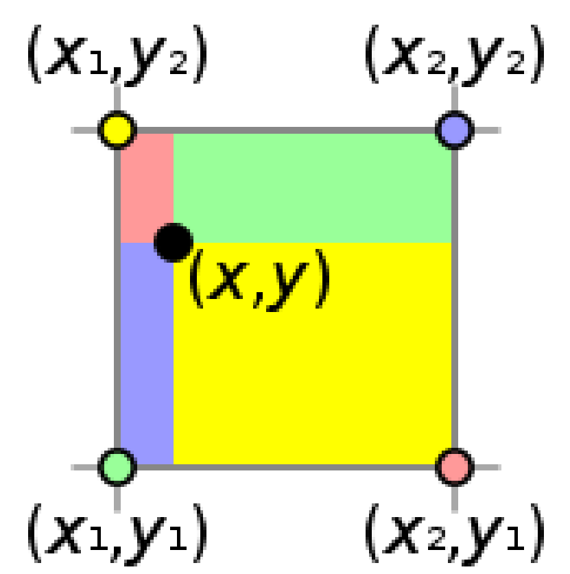
Bilinear Interpolation:
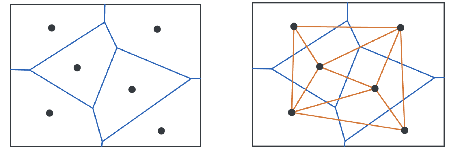
Delaunay Triangulation: Dual graph of Voroni Diagram
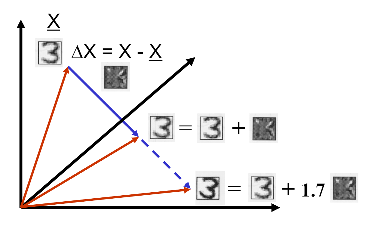
Morphing and Extrapolation

Lec 10: Cameras

Pinhole camera model
1. Defines Center of Projection (CoP) and Image Plane
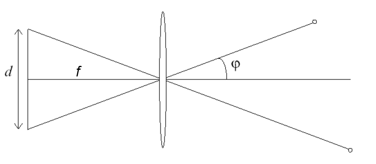
2. Defines Effective Focal Length as d
Camera coordinate systems
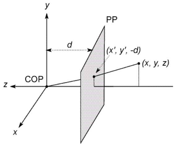
Projection:
1. Perspective Projection: $(x, y, z) \rightarrow (-d\frac{x}{z}, -d\frac{y}{z}, -d) \rightarrow (-d\frac{x}{z}, -d\frac{y}{z})$
2. Orthographic Projection: $(x, y, z) \rightarrow (x, y)$; special case when distance from COP to PP is infinite
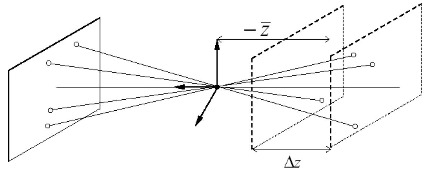
3. Weak Perspective/Orthographic: if $\Delta z << -\bar{z}, (x, y, z) \rightarrow (-mx, -my)$ where $m=-\frac{f}{\bar{z}}$
  
  Special case when scene depth is small relative to avg. distance from camera
  
  Equivalent to scale first then orthographic project
4. Spherical Projection: $(\theta, \phi) \rightarrow (\theta, \phi, d)$
Camera Parameters
1. Aperture: Bigger aperture = Shallower scene depth, Narrower gate width
2. Thin Lenses: $\frac{1}{d_o} + \frac{1}{d_i} = \frac{1}{f}$
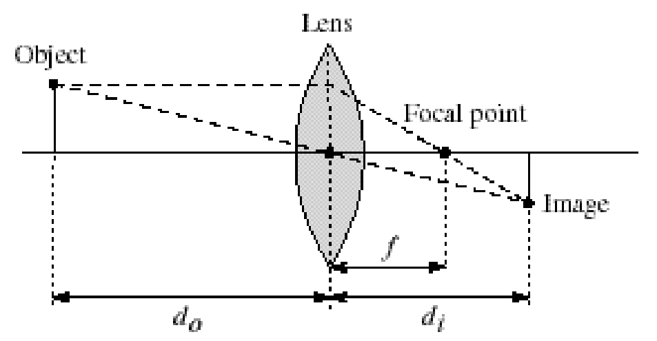
3. FOV (Field of View): $\phi = \tan^{-1}(\frac{d}{2f})$
4. Exposure & Shutter Speed
  1. Example: F5.6+1/30Sec = F11+1/8Sec
5. Lens Flaws
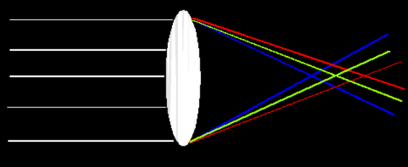
  1. Chromatic Aberration: Due to wavelength-dependent refractive index, modifies ray-bending and focal length
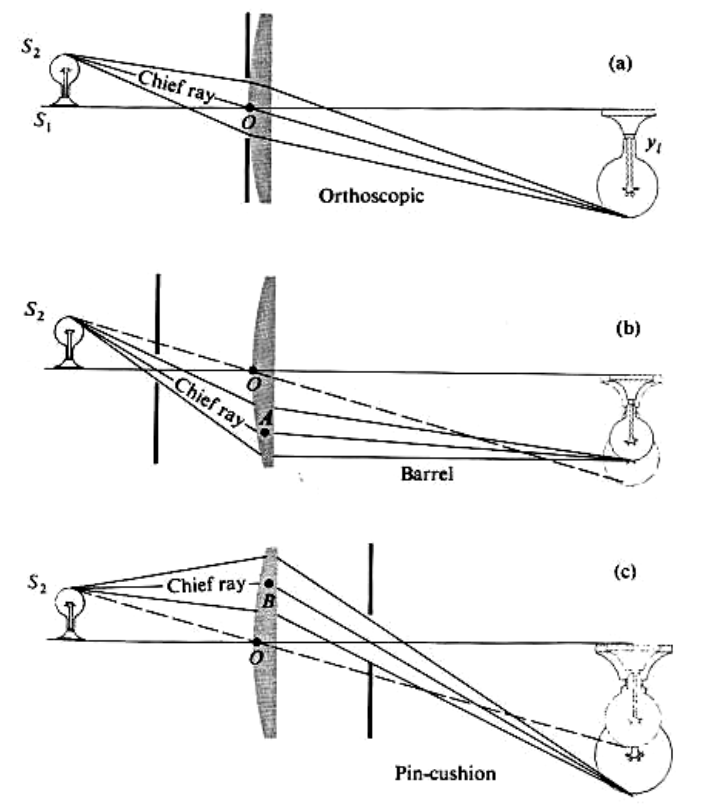
  2. Radial Distortion

Lec 11: Perspective Transforms

Formula: \[ H = \begin{pmatrix} a & b & c \\ d & e & f \\ g & h & 1 \end{pmatrix} \]

\[ \begin{pmatrix} x_1 & y_1 & 1 & 0 & 0 & 0 & -x_1 x_1' & -y_1 x_1' \\ 0 & 0 & 0 & x_1 & y_1 & 1 & -x_1 y_1' & -y_1 y_1' \\ x_2 & y_2 & 1 & 0 & 0 & 0 & -x_2 x_2' & -y_2 x_2' \\ 0 & 0 & 0 & x_2 & y_2 & 1 & -x_2 y_2' & -y_2 y_2' \\ \vdots & \vdots & \vdots & \vdots & \vdots & \vdots & \vdots & \vdots \\ x_N & y_N & 1 & 0 & 0 & 0 & -x_N x_N' & -y_N x_N' \\ 0 & 0 & 0 & x_N & y_N & 1 & -x_N y_N' & -y_N y_N' \end{pmatrix} \cdot \begin{pmatrix} a \\ b \\ c \\ d \\ e \\ f \\ g \\ h \end{pmatrix} = \begin{pmatrix} x_1' \\ y_1' \\ x_2' \\ y_2' \\ \vdots \\ x_N' \\ y_N' \end{pmatrix} \]

Solution: Least Squares, $x = (A^TA)^{-1}A^Tb$

Lec 12-14: Feature Extraction

Feature Detector:

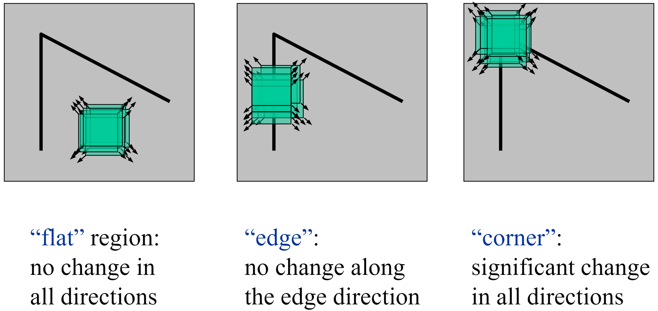
Change in appearance of window W for the shift $[u, v]$ is: \[ E(u, v) = \sum_{(x, y) \in W}[I(x+u, y+v) - I(x, y)]^2 \] Then, we use a First-order Taylor approximation for small motions $[u,v]$: \[ \begin{aligned} I(x+u, y+v) &= I(x, y) + I_x u + I_y v + \text{higher order terms} \\ &\approx I(x, y) + I_x u + I_y v \\ &= I(x, y) + \begin{bmatrix} I_x & I_y \end{bmatrix} \begin{bmatrix} u \\ v \end{bmatrix} \end{aligned} \]

\[ \begin{aligned} E(u, v) &= \sum_{(x, y) \in W} \left[I(x+u, y+v) - I(x, y)\right]^2 \\ &\approx \sum_{(x, y) \in W} \left[I(x, y) + \begin{bmatrix} I_x & I_y \end{bmatrix} \begin{bmatrix} u \\ v \end{bmatrix} - I(x, y)\right]^2 \\ &= \sum_{(x, y) \in W} \left(\begin{bmatrix} I_x & I_y \end{bmatrix} \begin{bmatrix} u \\ v \end{bmatrix}\right)^2 \\ &= \sum_{(x, y) \in W} \begin{bmatrix} u & v \end{bmatrix} \begin{bmatrix} I_x^2 & I_x I_y \\ I_x I_y & I_y^2 \end{bmatrix} \begin{bmatrix} u \\ v \end{bmatrix} \end{aligned} \]

This gives us the second moment matrix M, which is a approximate of local change on images. \[ M = \begin{bmatrix} I_x^2 & I_x I_y \\ I_x I_y & I_y^2 \end{bmatrix} \] Here, we calculate this function value as "corner strength": \[ R = \det(M) - k * \text{tr}(M)^2 \text{ or } \det(M)/\text{tr}(M) \] Remark: for flat areas, both $\lambda_1, \lambda_2$ are small; for edges, one of the $\lambda$ is big; for corners, both are big.
Scale Invariant Detection: choose the scale of best corner independently!
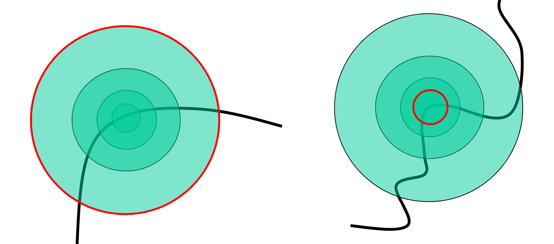
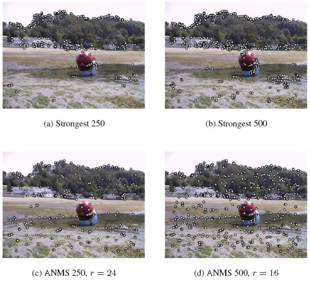
Feature Selection: ANMS
Feature Descriptor (Multi-scale Oriented Patches): 8x8 oriented patch, descripted by (x, y, scale, orientation)
1. Maybe normalized by $I' = (I-\mu)/\sigma$
Matching Feature:
1. Step 1: Lowe's Trick, match(1-NN) - match(2-NN)
2. Step 2: RANSAC (random choose 4 points; calc homography; calc outliers; finally select best homography)
Further Techniques: Order images to reduce inconsistencies

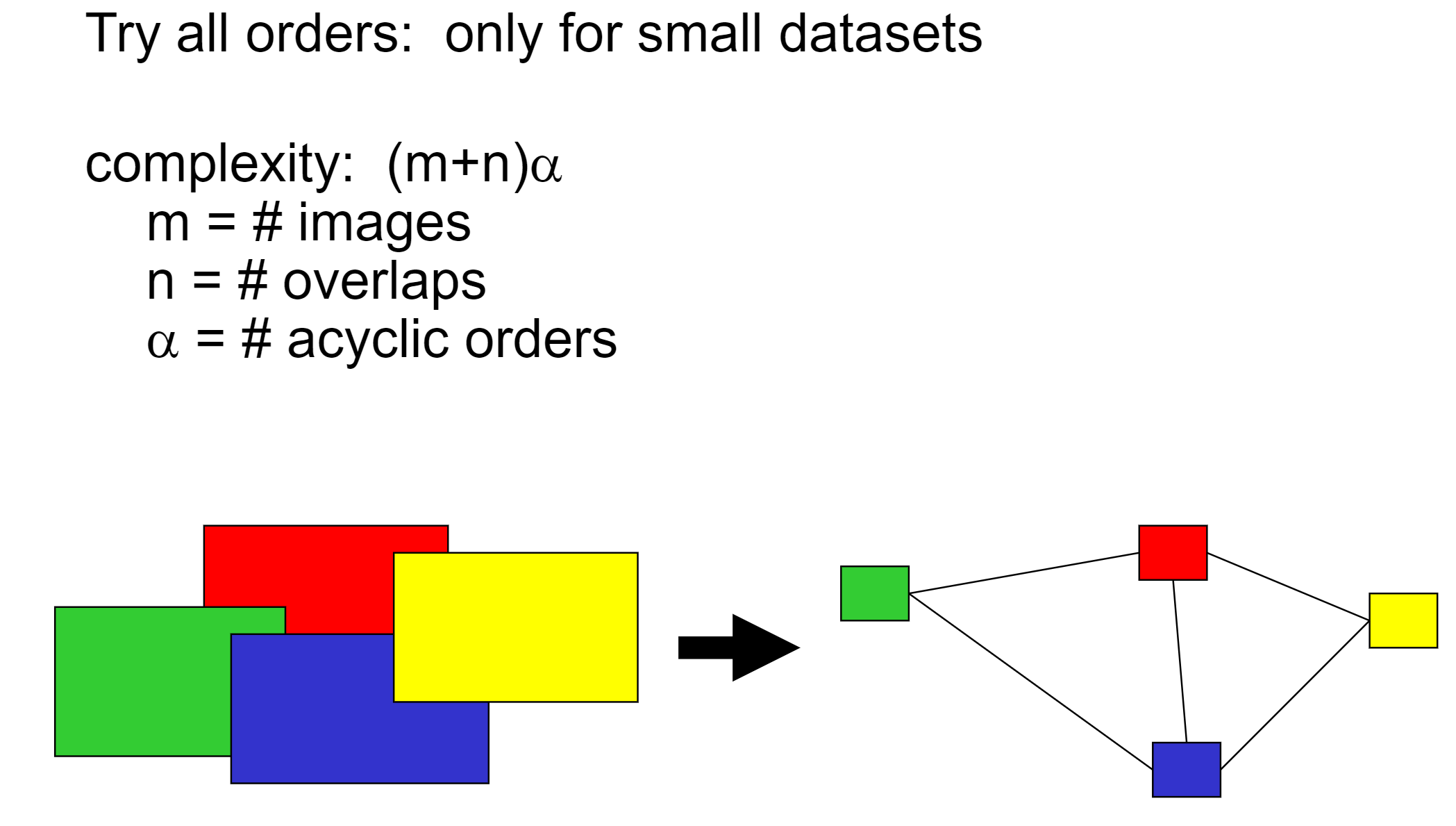
Do the loop: match images - order images - match images - ...
Optical Flow Algorithm \[ 0 = I(x+u, y+v)-H(x, y) \approx [I(x, y) - H(x, y)] + I_xu + I_yv = I_t + \nabla I \cdot [u, v] \] The component of the flow in the gradient direction is determined.

The component of the flow parallel to an edge is unknown.

To have more constraint, consider a bigger window size! \[ \begin{bmatrix} I_x(\mathbf{p}_1) & I_y(\mathbf{p}_1) \\ I_x(\mathbf{p}_2) & I_y(\mathbf{p}_2) \\ \vdots & \vdots \\ I_x(\mathbf{p}_{25}) & I_y(\mathbf{p}_{25}) \end{bmatrix} \begin{bmatrix} u \\ v \end{bmatrix} = - \begin{bmatrix} I_t(\mathbf{p}_1) \\ I_t(\mathbf{p}_2) \\ \vdots \\ I_t(\mathbf{p}_{25}) \end{bmatrix} \] Solve by least square: (Lukas & Kanade, 1981) \[ (A^T A) \mathbf{d} = A^T \mathbf{b} \]

\[ \begin{bmatrix} \sum I_x I_x & \sum I_x I_y \\ \sum I_x I_y & \sum I_y I_y \end{bmatrix} \begin{bmatrix} u \\ v \end{bmatrix} = - \begin{bmatrix} \sum I_x I_t \\ \sum I_y I_t \end{bmatrix} \]

This is solvable when: no aperture problem.

How to make it even better? Do it multi-hierachical!

Lec 15-16: Texture Models

Human vision patterns
1. Pre-attentive vision: parallel, instantaneous (~100--200ms), without scrutiny, independent of the number of patterns, covering a large visual field.
2. Attentive vision: serial search by focal attention in 50ms steps limited to small aperture.
Order statistics of Textures
1. Textures cannot be spontaneously discriminated if they have the same first-order and second-order statistics of texture features (textons) and differ only in their third-order or higher-order statistics.
2. First order: mean, var, std, ...
3. Second order: co-occurence matrix, contrast, ...
Introduction: Cells in Retina
1. Receptive field of a retinal ganglion cell can be modeled as a LoG filter. (Corner Detectors)
2. Cortical Receptive Fields -> (Line/Edge Detectors)
3. They are connected just like a CNN network.
From Cells to Image Filters: [Filter Banks]

Detects Statistical unit of texture (texton) in real images:

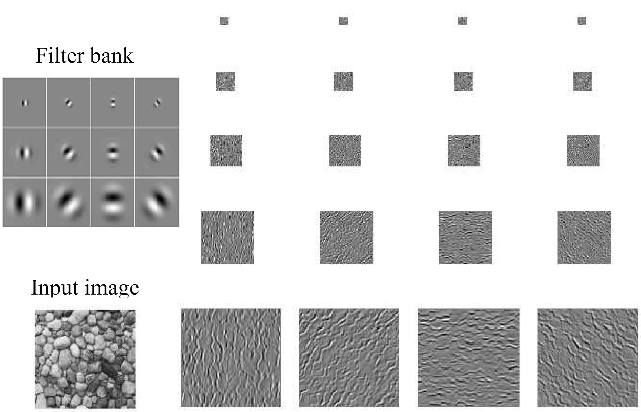
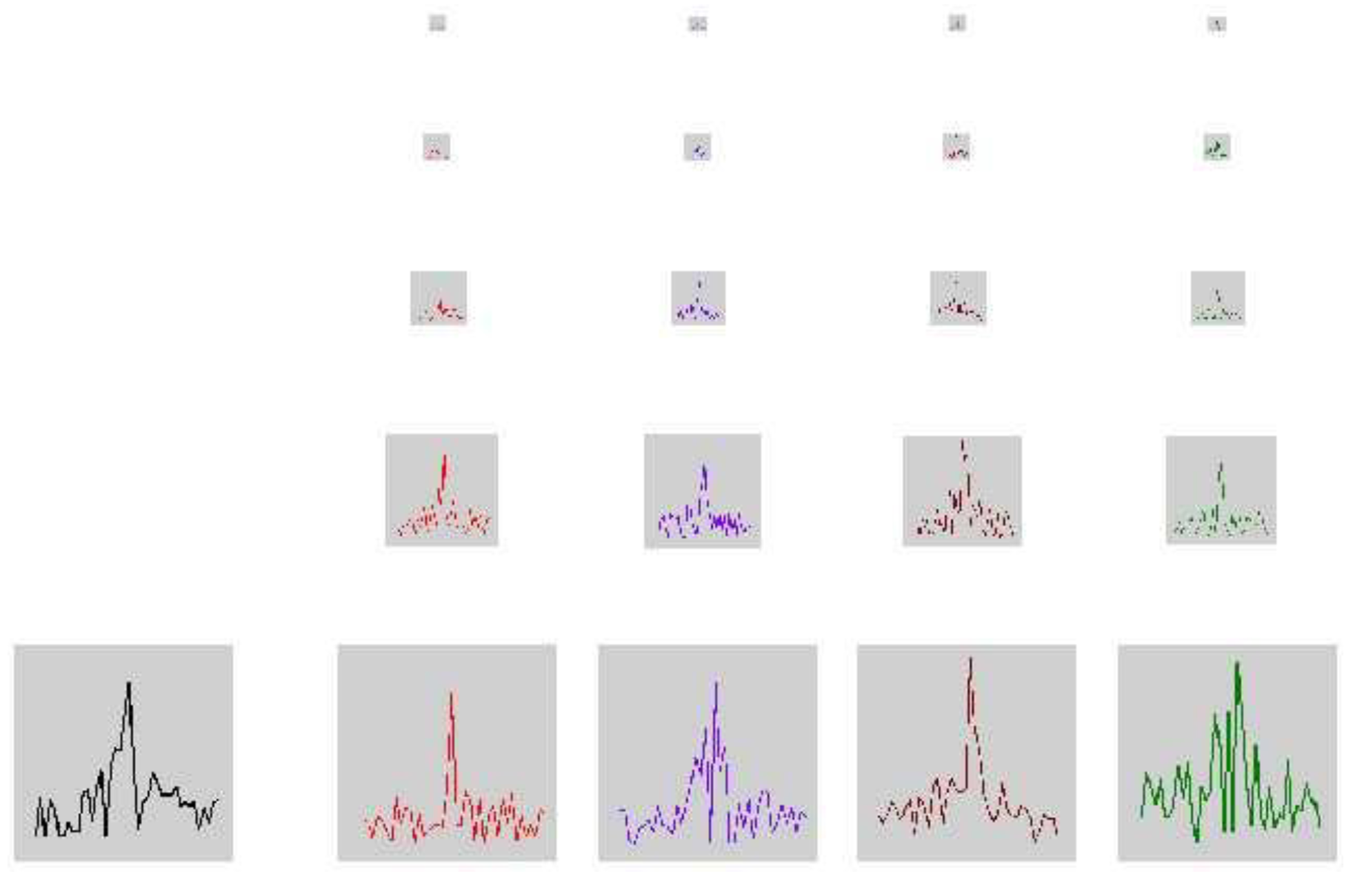
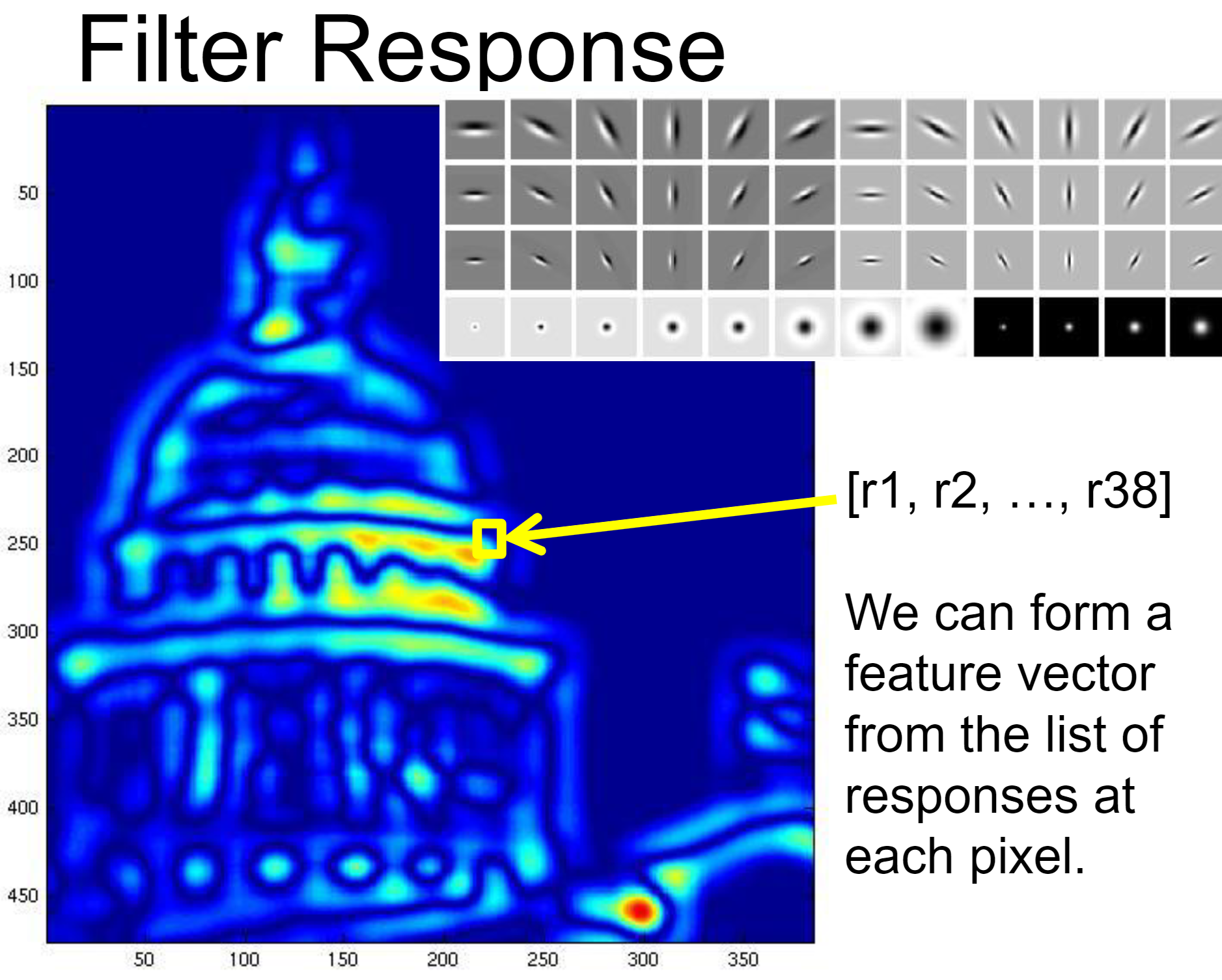
Texton summary: from object to bag of "words"; Preliminaries of CNN
Image Feature Repr:
1. Code Words -> Hist Matching
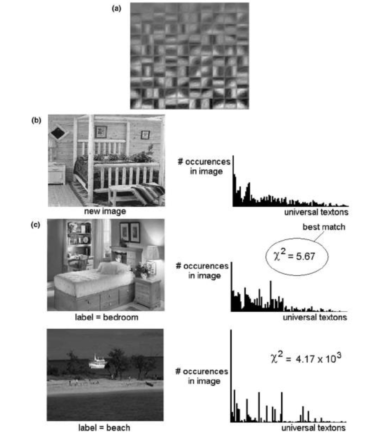
Image-2-Image Translation
1. Target: Depths, Normals, Pixelwise-Segmentation/Labelling, Grey-2-Color, Edges-2-Photo, ...
2. Wrong exmples:
  1. Stacking $2n+1$ convolutions (receptive fields) for $n$ pixels: too many convolutions!
  2. Extract NxN patches and independently do CNN: requires too much patches
3. Answer: Encoder+Decoder, Convolutions and Pooling
4. How about missing details when up-sampling? Copy a high-resolution Version! (U-Net)
5. How about loss function? L2 don't work for task: image colorization
  1. Use per-pixel multinomial classification! (Some what like a bayes net P(label1|pix1), P(label2|pix1), ...)
  2. $L(\mathbf{\hat{Z}}, \mathbf{Z}) = -\frac{1}{HW}\sum_{h,w}\sum_{q}\mathbf{Z}_{h,w,q}\log(\mathbf{\hat{Z}}_{h,w,q})$ where q is probability of label q; This is a cross-entropy.
Universal loss for Img2Img Tasks: GAN
1. Structure: Input -> Generator -> Generated Im; G(x) -> Discriminator -> Loss (Represented as probability; Suppose D(x) is prob that x is fake)
2. D's task: $\arg \max_D \mathbb{E}_{x, y}[\log D(G(x)) + \log(1-D(y))]$
3. G's task:
  1. Tries to synthesize fake images that fool D: $\arg \min_G \mathbb{E}_{x, y}[\log D(G(x)) + \log(1-D(y))]$
  2. Tries to synthesize fake images that fool the best D:
    
    $\arg \min_G \max_D \mathbb{E}_{x, y}[\log D(G(x)) + \log(1-D(y))]$
4. Training Process:
  1. Sample $x \sim p_{data}, z \sim p_z$
  2. Calc $L_D$ and backward
  3. Calc $L_{G}$ and backward
5. Example Img2Img Tasks: Labels->Facades, Day->Night, Thermal->RGB, ...

Lec 17-18: Generative Models

Revision of an Early Vision Texture Model:
1. Select $x \sim p_{data}; z \sim p_z$ (z is usually noise)
2. Multi-scale filter decomposition (Convolve both images with filter bank)
3. Match per channel histograms (from noise to data)
4. Collapse pyramid and repeat
Make it better?
1. Match joint histograms of pairs of filter responses at adjacent spatial locations, orientations, scales, ...
2. Optimize using repeated projections onto statistical constraint surfaces.
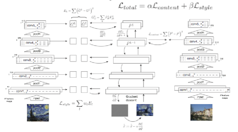
Make it more modern: Use CNN to do texture synthesis
1. Previously, we use histograms to describe texture features. Now, we use Gram Matrices on CNN Features as texture features.
  
  Define CNN output of some layer as: \[ F_{N\times C} = [f_1, f_2, \dots, f_N]^T \] We have: \[ G = FF^T = \begin{bmatrix} \langle f_1, f_1 \rangle & \cdots & \langle f_1, f_N \rangle \\ \vdots & & \vdots \\ \langle f_N, f_1 \rangle & \cdots & \langle f_N, f_N \rangle \end{bmatrix} \] where \[ \langle f_i, f_j \rangle = \sum_k F_{ik} F^T_{kj} \] This describes the correlation of image feature $f_i$ and $f_j$, which are both length C (channel) vectors.
2. Define loss as: \[ L_{\text{style}} = \sum_l \frac{1}{C_l^2 H_l^2 W_l^2} \| G_l(\hat{I}) - G_l(I_{\text{style}}) \|_F^2 \]
3. Pipeline for Texture Synthesis:
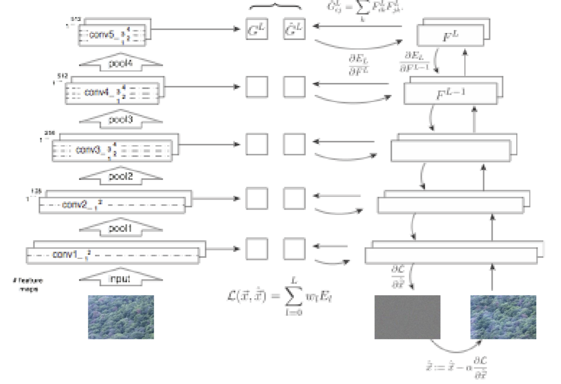
4. Remark: The CNN used here is just a pre-trained texture-recognition CNN network, where VGG-16 or VGG-19 nets can be used.
  
  Basically, select any CNN network that is trained to map from image to label (e.g. "dog") will recognize features totally fine. They are already trained on ImageNet dataset.
Use CNN to do artistic style transfer
1. Loss Function Design:
  1. \[ L_{\text{style}} = \sum_l \frac{1}{C_l^2 H_l^2 W_l^2} \| G_l(\hat{I}) - G_l(I_{\text{style}}) \|_F^2 \]
  2. \[ L_{\text{content}} = \frac{1}{2} \sum_{i,j} \left( F_{i,j}^{\text{generated}} - F_{i,j}^{\text{content}} \right)^2 \]
2. Pipeline:
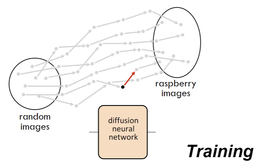
Diffusion
1. Training / Inference(Forward):
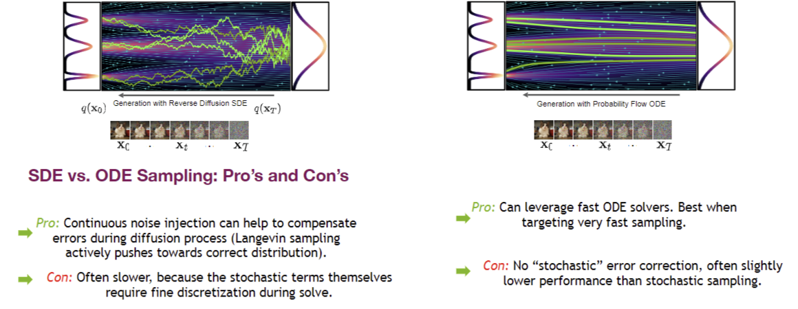
2. Sampling methods: DDPM vs DDIM
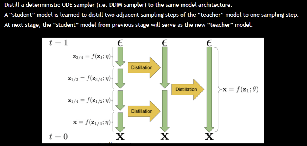
3. Make sampling faster? Distilation!
4. Editing desired area? Generate a mask that a word corresponds to!
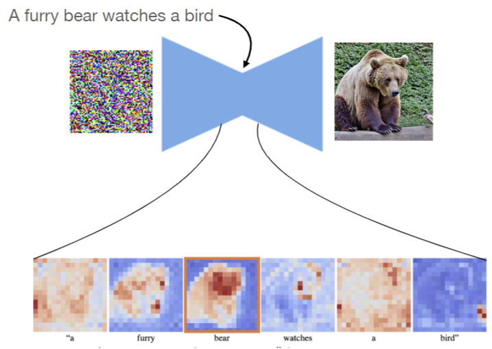
Common Image Generating Models:
1. Parti: self-regressive model; generates images block by block
2. Imagen: Diffusion
3. Dalle-2: Parti + Imagen

Lec 19: Sequence Models

Shannon, 1948: N-gram model; Compute prob. dist. of each letter given N-1 previous letters (Markov Chain)
Video Textures, Sig2000:
1. Compute L2 distance $D_{i, j}$ for between all frames
2. Markov Chain Repr
3. Transition costs: $C_{i \rightarrow j} = D_{i+1, j}$; Probability Calculated as: $P_{i \rightarrow j} \propto \exp(-C_{i \rightarrow j} / \sigma^2)$
4. Problem: Preserving Dymanics? Solution: Use previous N frames to calculate cost.
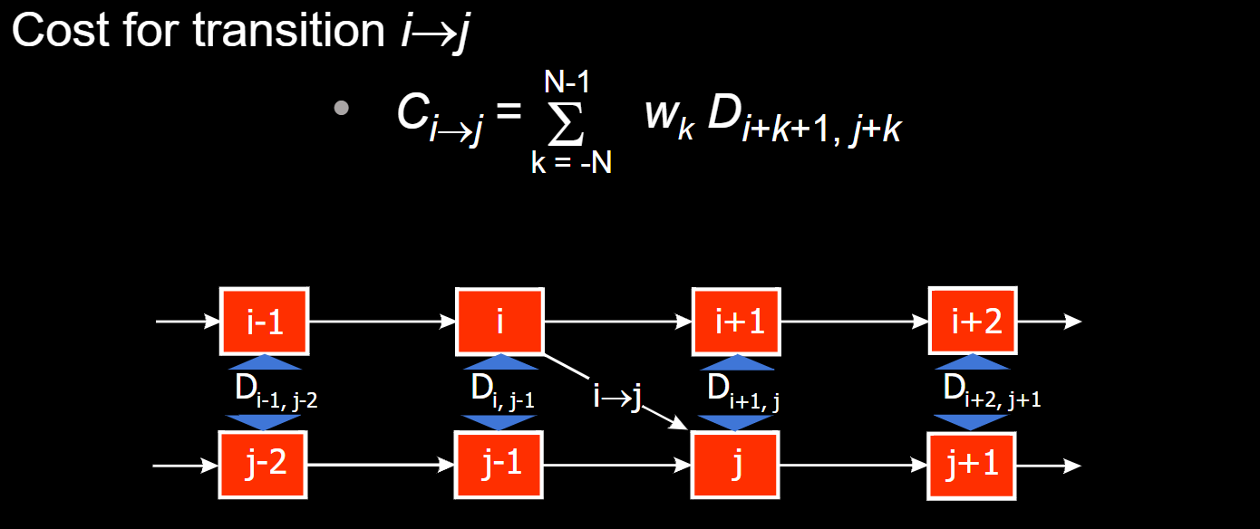
5. Problem: Control video texture speed? Solution: change the weighted sum parameters of previous N costs.
6. Problem: User control? (e.g. fish chasing mouse pointer)? Solution: add user control term $L = \alpha C + \beta \text{angle}$
  1. Maybe need to precompute future costs for a few angles
Efros & Leung Texture Synthesis Algorithm:

(Bigger window size is better, but requires more params!)
Image Analogies Algorithm: Process an image by example (A:A' :: B:B') (Siggraph 2001)
1. Compare area of pixels (e.g. 10*10) from img A and B.
2. Find the best match, then copy some smaller area of pixels (e.g. 3*3) from imgA' to imgB'
3. Remark: Neurips 2022, later method uses VQ-GAN and MAE to finish this
Word Embedding (word2Vec, GloVe)...
Attention + Prediction: Word sequence tasks
1. possible explanation: different layers (attention+prediction) works for different functions (syntax, semantics, ...)
Similar methods for image generation: treat image as blocks of pixels and generate in order (Parti)

Lec 20: Single View 3D Vision Geometry

Projecting points: use homo coords $(sx, sy, s)$
Projecting lines:
1. A line in the image correspond to a plane of rays through origin.
2. Computing vanishing points:
  
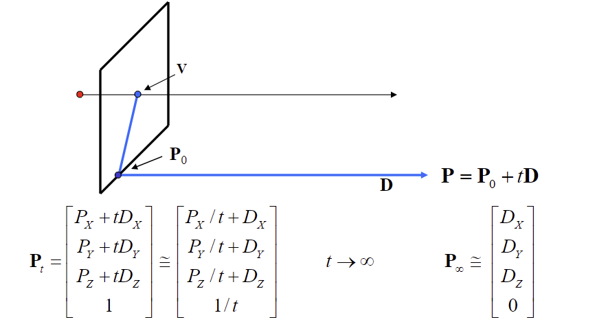
  Remark1: Any two parallel lines have same vanishing point.
  
  Remark2: An image may have more than one vanishing point.
3. The union of all vanishing points is the horizon line (vanishing line)
  
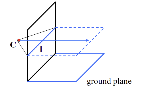
  Different planes define different vanishing lines
  
  Compute from two sets of parallel lines on the ground plane
  
  All points at same height as C projects to I
3D from single image
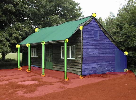
1. Find world coordinates (X, Y, Z) for a few points.
  1. Define ground plane (Z=0)
    
    Detecting lines in image? Use Hough Transform
  2. Compute points (X,Y,0) on that plane (by homography)
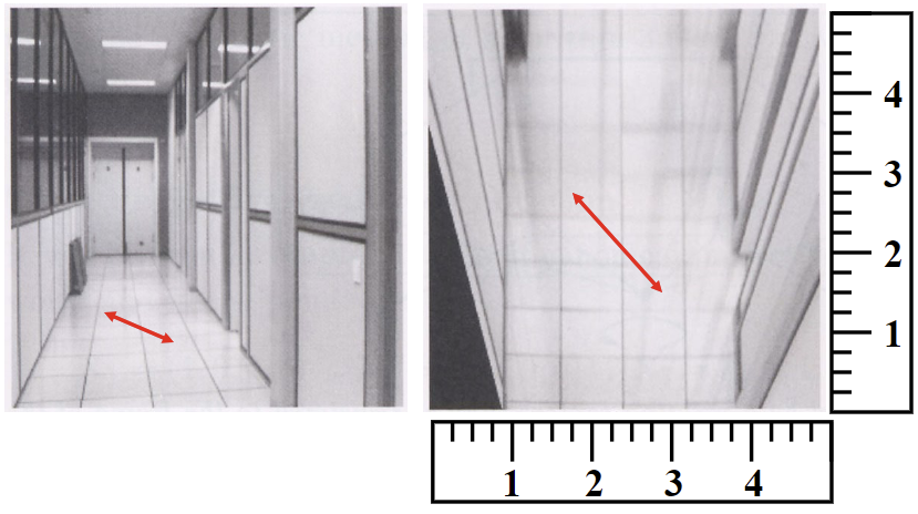
  3. Compute the heights Z of all other points (using perspective clues)

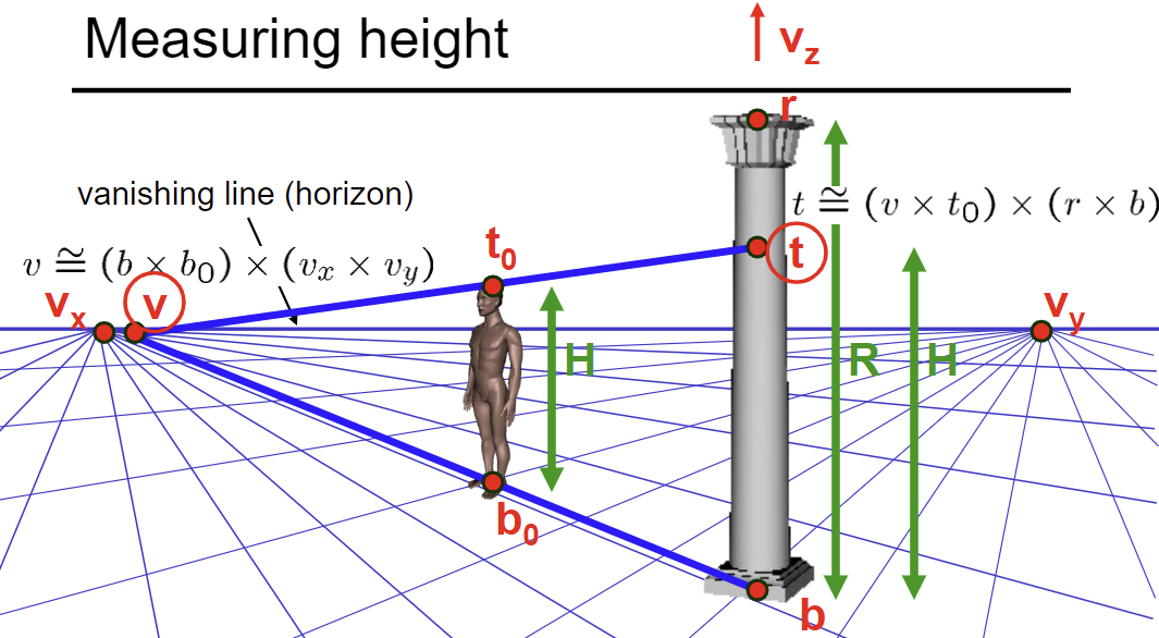
Lec 21: Multiple View 3D Geometry

Disparity Map * Depth Map = Constant.
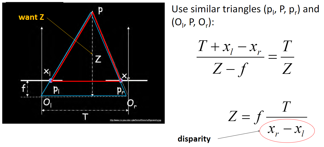
Correspondence problem:
1. Calculate Epipolar; Match along epipolar line
2. Effect of window size: want window large enough to have sufficient intensity variation, yet small enough to contain only pixels about the same disparity
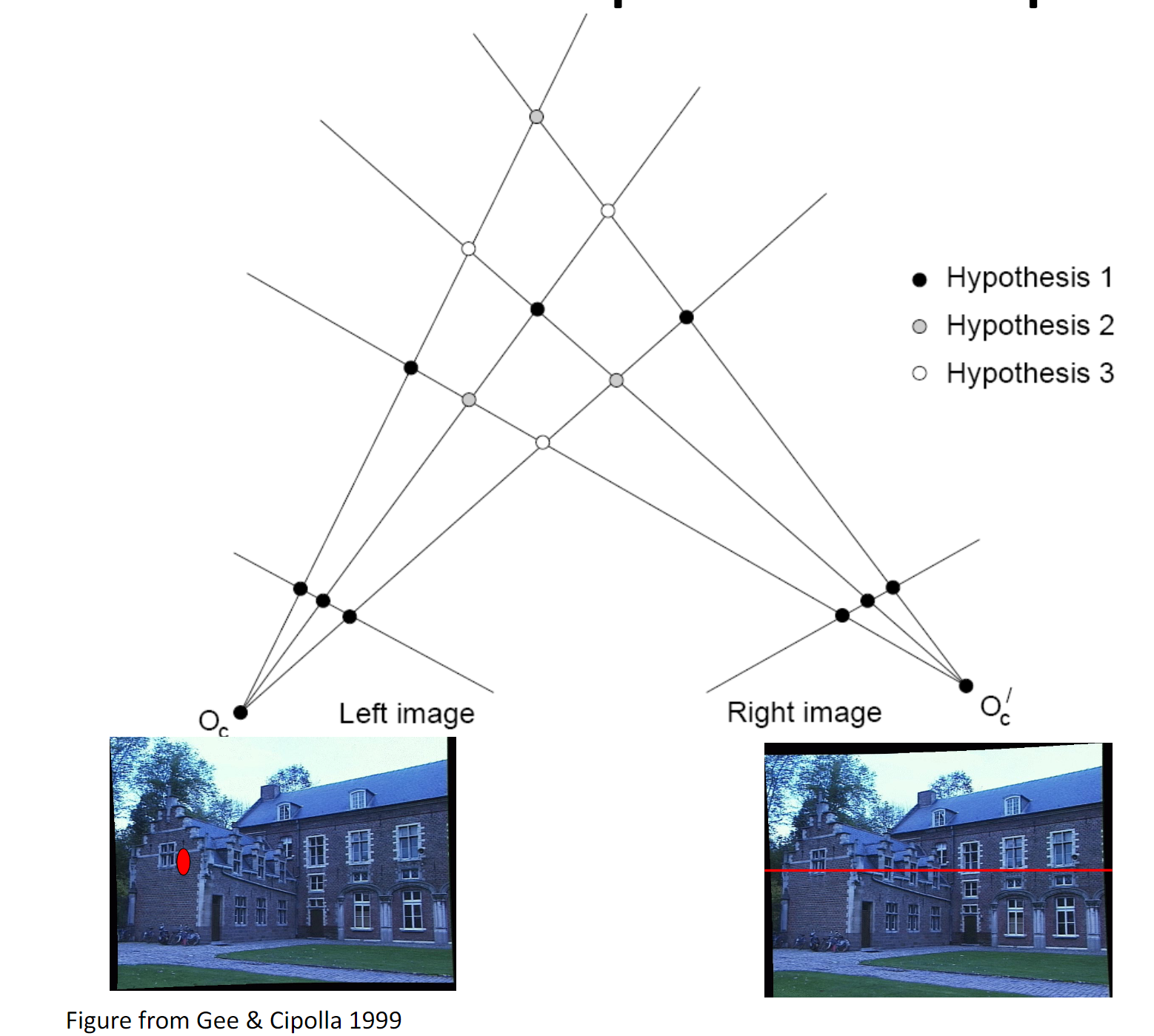
Feature Correspondence Pipeline:
1. Detect Keypoints; 2. Extract SIFT at each keypoint; 3. Finding correspondences
2. ALSO: CNN-based stereo matching / depth(disparity) estimation
  1. Feature Extraction; Calculate Cost Volume (pixel i's matching cost at disparity d); Cost Aggregation; Disparity Estimate (simple argmin)
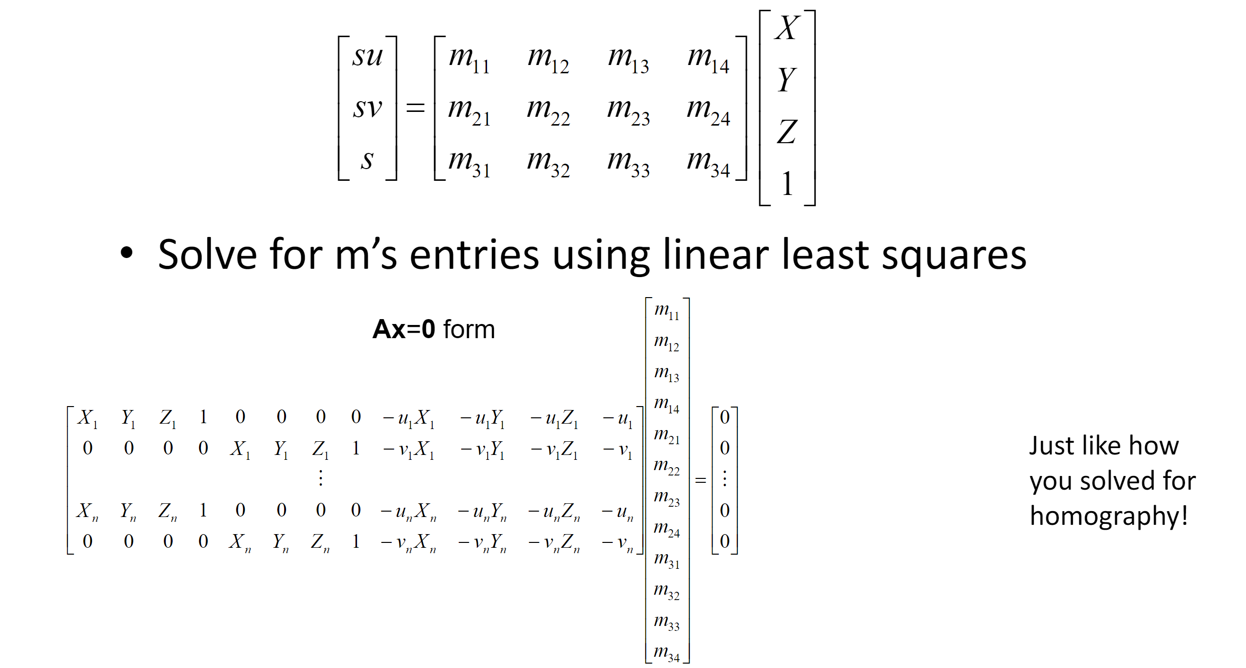
Camera Projection Model: $x_{uv} = K[R, t]X_{xyz}$ where $[R, t]$ is w2c matrix
Calibrate a Camera? Learning Problem. (use least square; just like solving homography)

Once we have solved M, decomposite it to K*R using RQ decomposition.
Epipolar Geometry:
1. Introduction: Camera may have rotation, along with translation
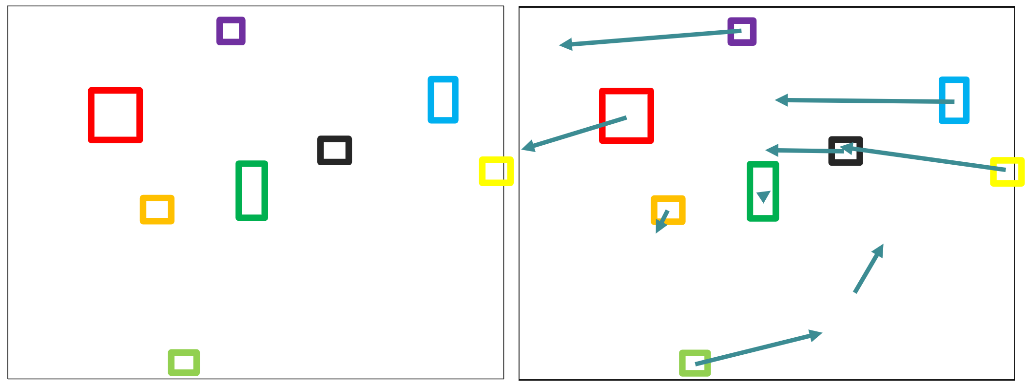
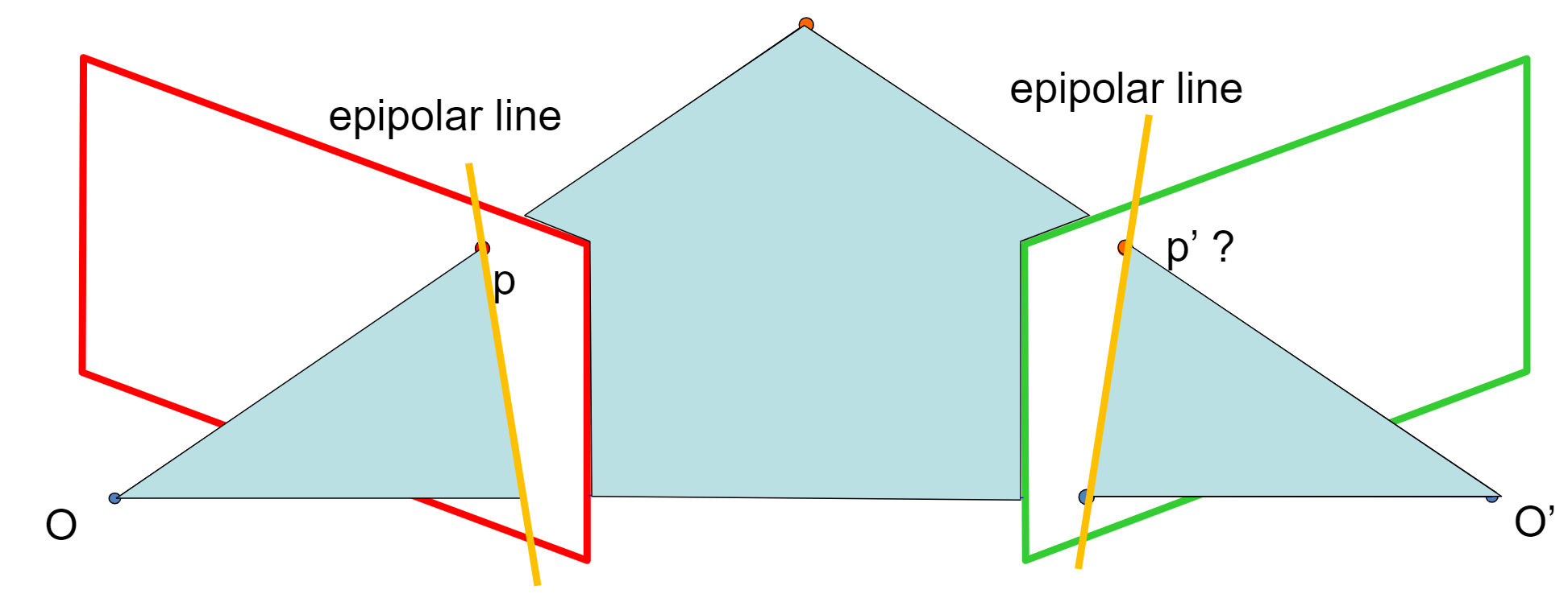
2. Definitions
  
  Baseline: the line connecting the two camera centers
  
  Epipole: point of intersection of baseline with the image plane
  
  Epipolar plane: the plane that contains the two camera centers and a 3D point in the world
  
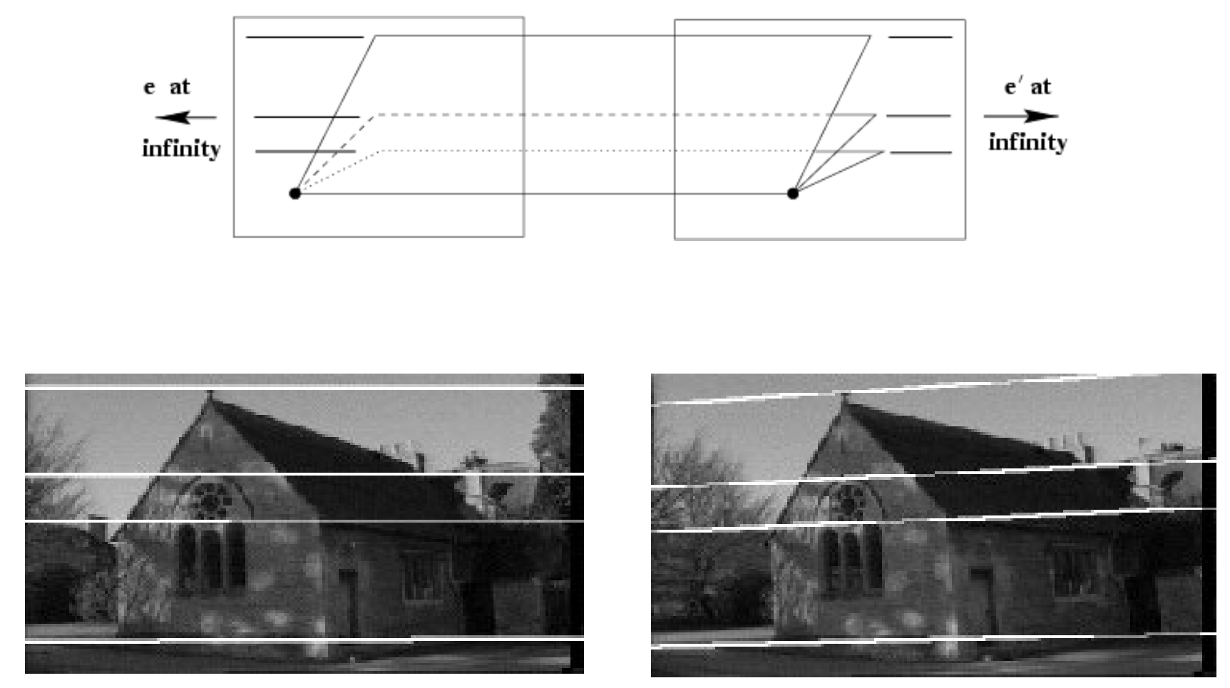
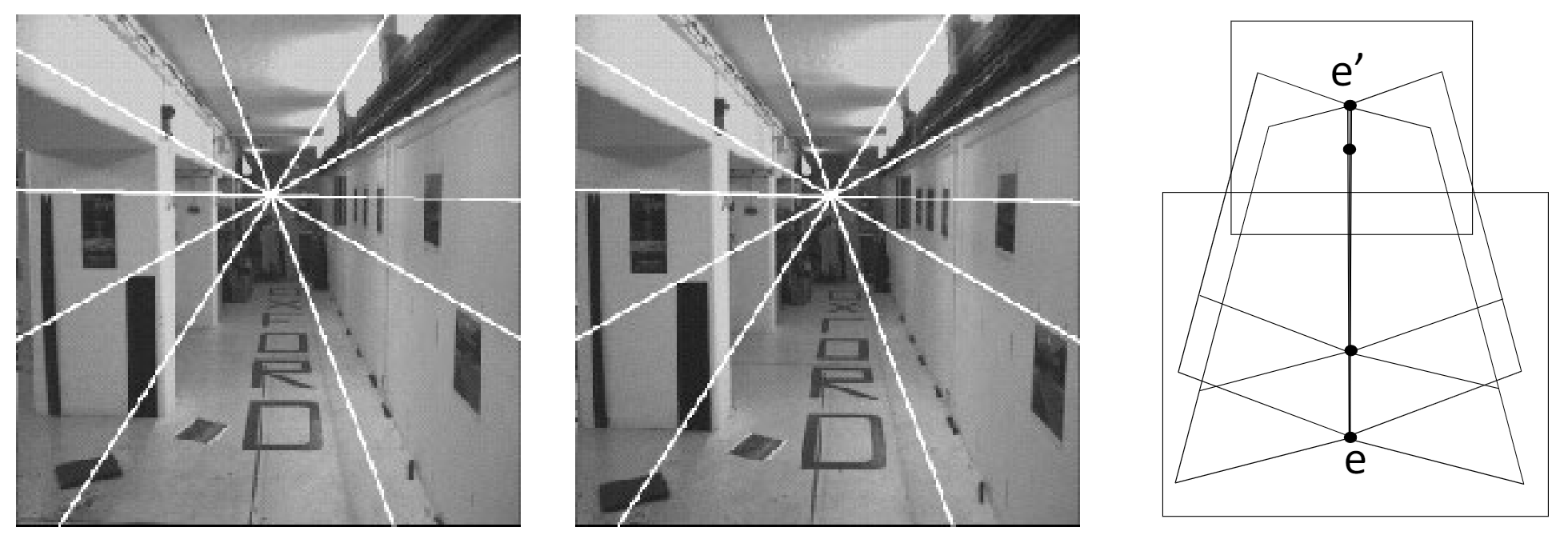
  Epipolar line: intersection of the epipolar plane with each image plane
  
  EXAMPLE 1: parallel movement
  
  EXAMPLE 2: forward movement
3. Usage: Stereo image rectification
  
  Reproject image planes onto a common plane parallel to the line between optical centers
  
  Then pixel motion is horizontal after transformation
  
  Two homographies (3x3 transforms), one for each input image reprojection
4. Calculations: How to express epipolar constraints? (When camera is calibrated)
  
  Answer: use Essential Matrix
  
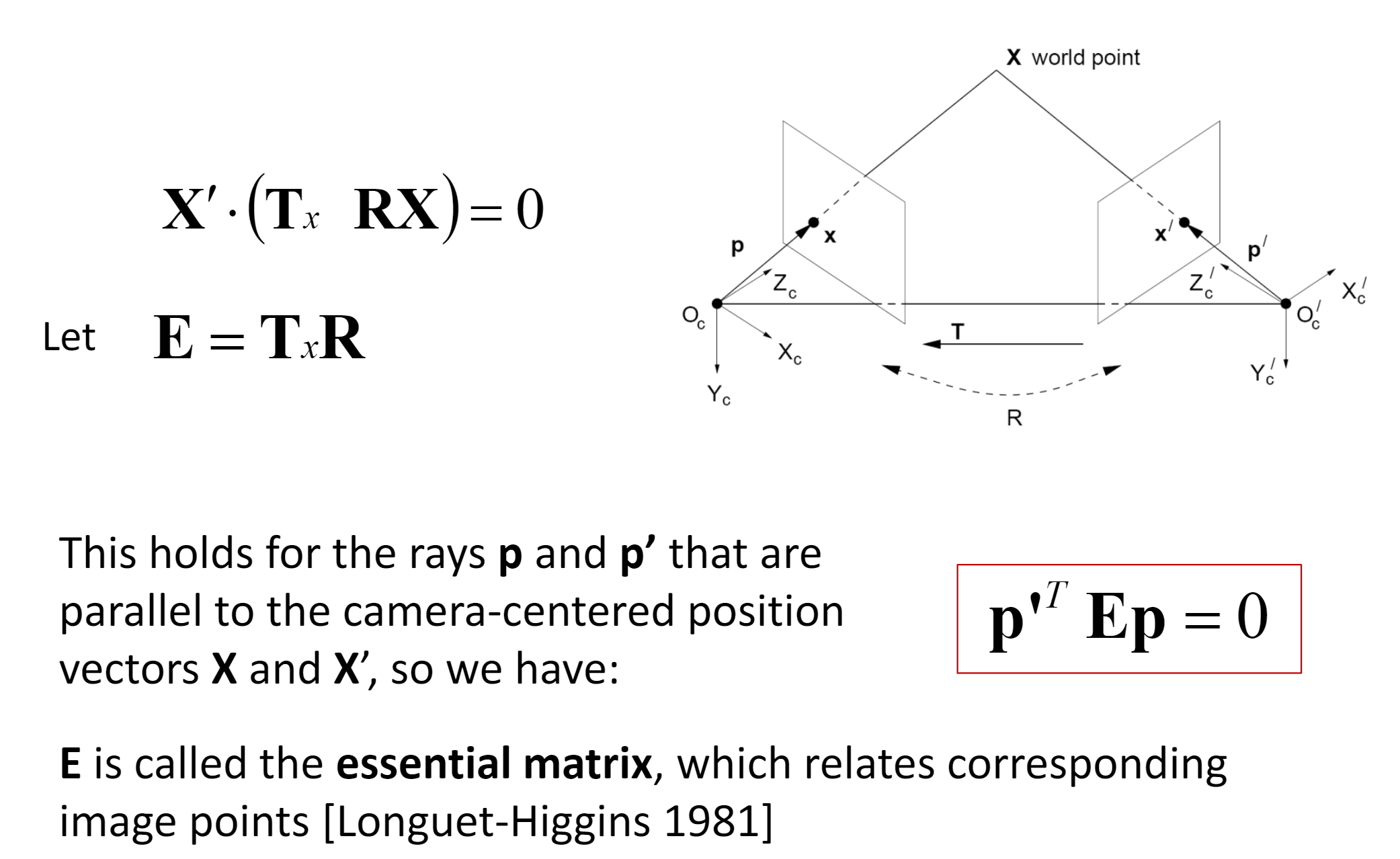
  Proof: $X'=RX+T; T \times X' = T \times RX + T \times T = T \times RX; X' \times (T \times X') = 0$
  
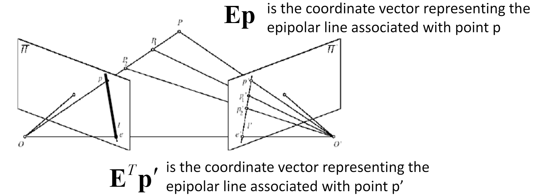
  Properties of $E=T_xR$:
  - $ Ex' $ is the epipolar line associated with $ x' $ ($ l = E x' $)
  - $ E^Tx $ is the epipolar line associated with $ x $ ($ l' = E^T x $)
  - $ E e' = 0 $ and $ E^T e = 0 $
  - $ E $ is singular (rank two)
  - $ E $ has five degrees of freedom (3 for rotation $ R $, 2 for translation $ t $ since it is up to a scale)
5. Calculations: How to express epipolar constraints? (When camera is un-calibrated)
  
  Answer: Estimate the Fundamental matrix.
  
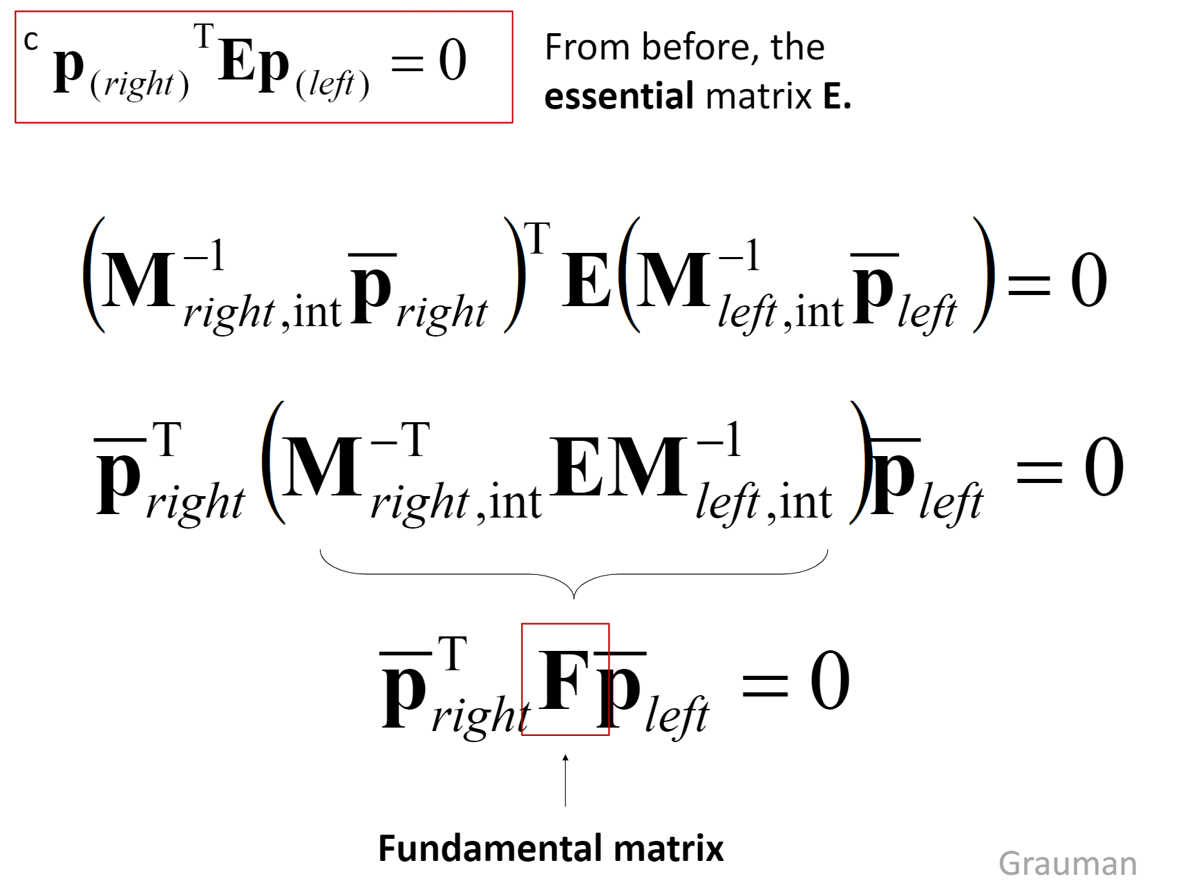
  Estimate F from at least 8 corresponding points
  
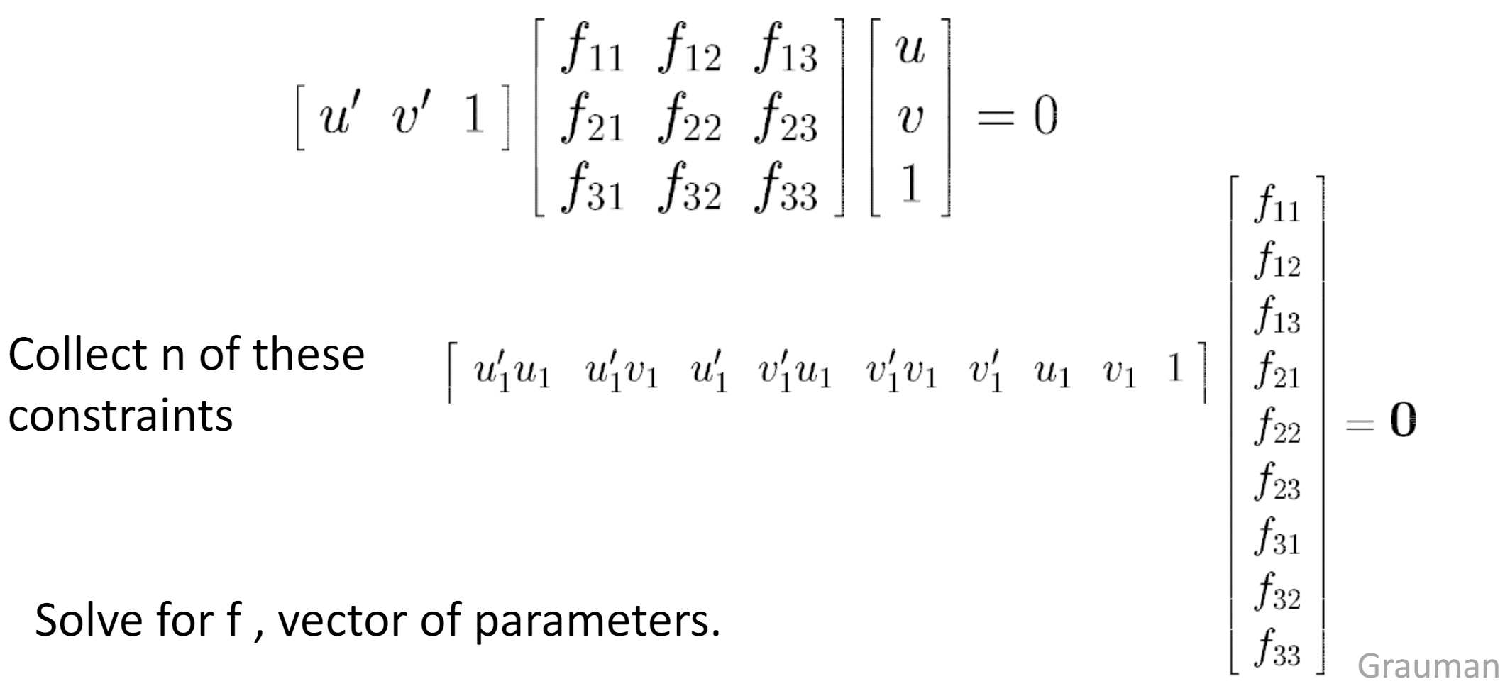
  *: Rank constrain: must do SVD on F and throw out the smallest singular value to enforce rank-2 constraint

Lec 22: SFM, MVS

Problem: unknown 3D Points, Correspondences, Camera Calibration
Solution:
1. Feature Detection; Matching between each pair using RANSAC;
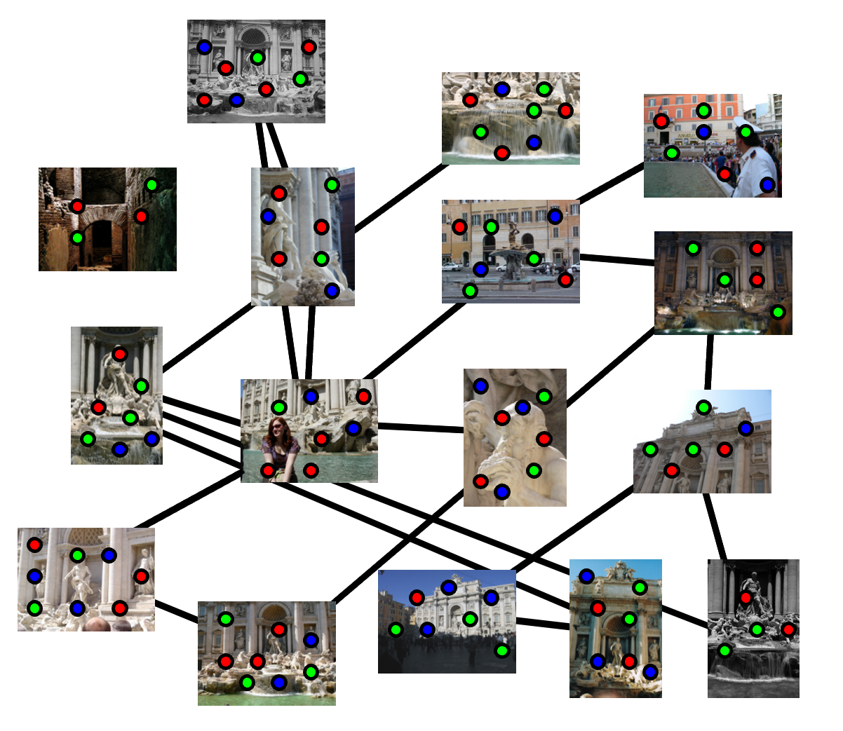
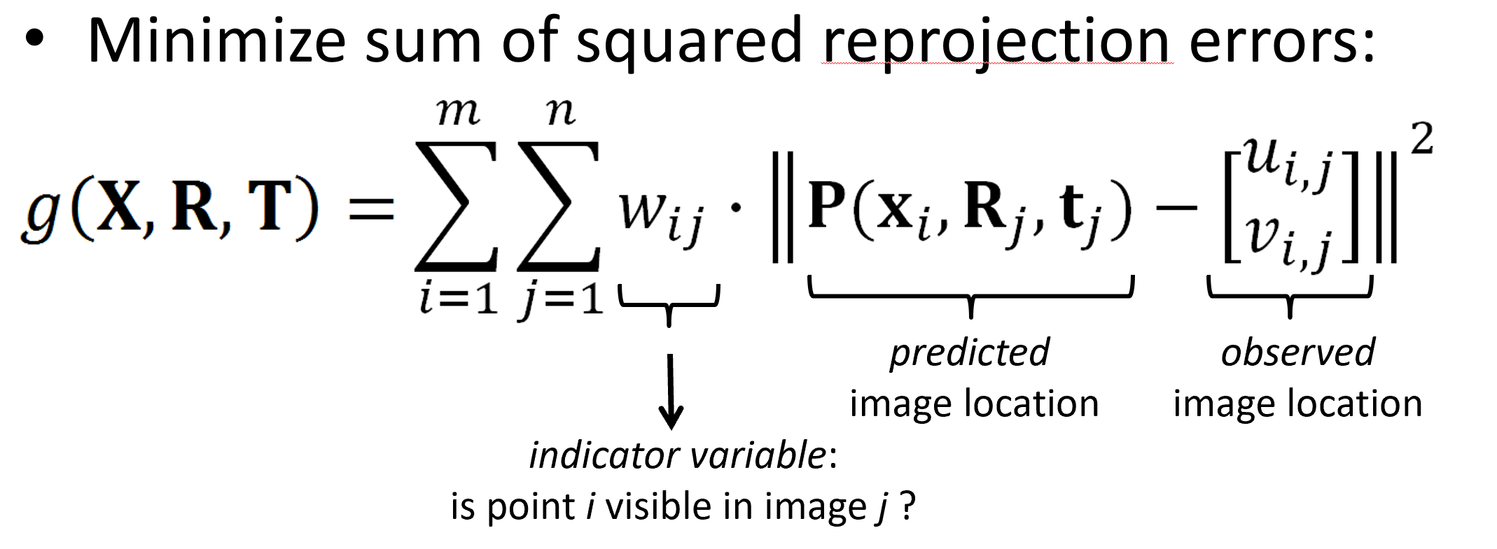
2. Calculate SFM using Bundle Adjustment; Optimized using non-linear least squares (E.g. Levenberg-Marquardt)
3. Problem: hard to init all cameras;
  
  Solution: only start with 1/2 cameras, then grow (kind of online algorithm); "Incremental SFM"
  1. Choose a pair with many matches and as large a baseline as possible
  2. Initialize model with two-frame SFM
  3. While there are connected images remaining, pick one that sees the most existing 3D points; estimate pose; triangulate new points; run bundle adjustment