
UC-Berkeley 24FA CV Project 1: Colorizing the Images of the Russian Empire
RoadMap
This project involves two parts:
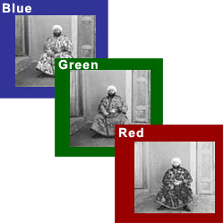
1. Colorize the image by aligning the
mismatched RGB channels separately.
2. Fix the color issues with Auto-Contrasting &
WhiteBalancing
Background
Sergei Mikhailovich Prokudin-Gorskii (1863-1944) was a man well ahead
of his time. Convinced, as early as 1907, that color photography was the
wave of the future, he won Tzar's special permission to travel across
the vast Russian Empire and take color photographs of everything he saw
including the only color portrait of Leo Tolstoy. And he really
photographed everything: people, buildings, landscapes, railroads,
bridges... thousands of color pictures!
His idea was simple: record three exposures of every scene onto a glass
plate using a red, a green, and a blue filter. Never mind that there was
no way to print color photographs until much later -- he envisioned
special projectors to be installed in "multimedia" classrooms all across
Russia where the children would be able to learn about their vast
country. Alas, his plans never materialized: he left Russia in 1918,
right after the revolution, never to return again.
Luckily, his RGB glass plate negatives, capturing the last years of the
Russian Empire, survived and were purchased in 1948 by the Library of
Congress. The LoC has recently digitized the negatives and made them
available on-line.
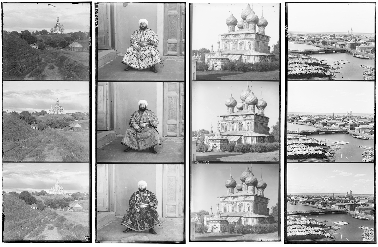
Image Aligning
Preprocessing: Removing Borders
- We start by calculating the average values both horizontally and
vertically, resulting in a
[H, 1]matrix and a[1, W]matrix. - Next, we remove the outermost white border and the second outermost black border using a threshold.
Single-Layer Image Aligning
Firstly, we align low-resolution images by exhaustively searching over a window of possible displacements, score each one using some image matching metric, and take the displacement with the best score. This is rather brute-force, but the low-resolution makes the calculation time acceptable.
A good metric to asses the similarity of two pictures is crucial. Traditional Euclidian Distances aren't good ideas, since different channels don't necessarily have same features like average brightness, variance, etc.
Here we choose SSIM as our assessment function. SSIM is defined as a product of 3 parts: Lightness part, Contrast part and Structural part. Here is a visualized result why SSIM is better than Euclidean Distance:
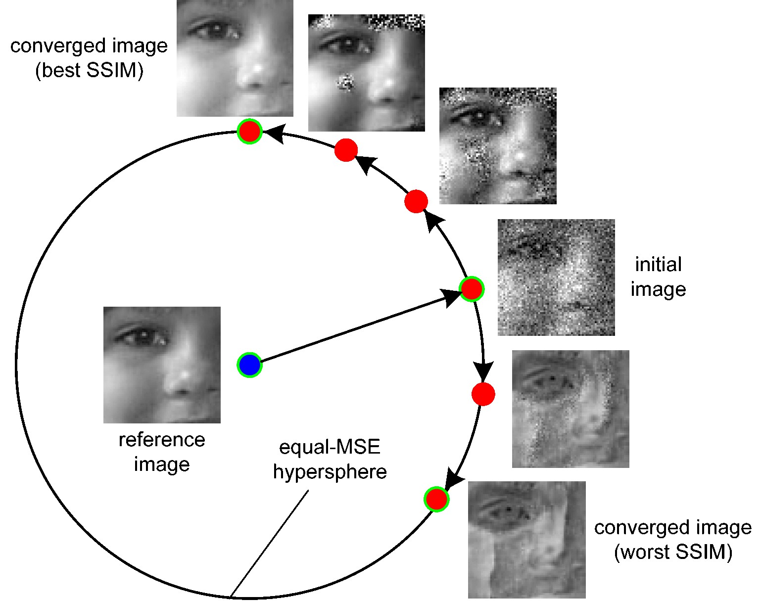
Figure 1: equal-MSE hypersphere from cns.nyu.edu/~lcv/ssim/
\[ \text{SSIM}(x, y) = l(x, y)^\alpha \cdot c(x, y)^\beta \cdot s(x, y)^\gamma \\ \]
\[ \begin{aligned} l(x, y) &= \frac{2\mu_x\mu_y + C_1}{\mu_x^2 + \mu_y^2 + C_1} \\ c(x, y) &= \frac{2\sigma_x\sigma_y + C_2}{\sigma_x^2 + \sigma_y^2 + C_2} \\ s(x, y) &= \frac{\sigma_{xy} + C_3}{\sigma_x\sigma_y + C_3} \end{aligned} \]
Remark: Introduce the constant \(C_1, C_2, C_3\) to avoid zero division. Usually a tiny number.
Multiscale Image Aligning
Although the basic method works for low-resolution images, it usually fails for larger images due to the workload increasing with \(O(n^2)\). To address this, we use an image pyramid approach, which combines both low-resolution (down-sampled) and high-resolution (original) versions of the image. This allows us to handle the problem iteratively: we first align the smallest image, then transfer the resulting offsets to progressively larger images, aligning each one in turn. Specifically, this approach uses a stack structure.
- Initially, a
whilelooppushes images, each halved in size from the previous one, into thestack. - In each iteration, the loop
pops the last image from the stack and aligns it. - The resulting offset is then doubled and applied to the next higher-resolution image in the subsequent loop iteration.
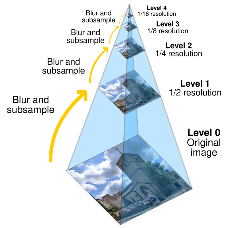
Figure 2: image pyramid from Pyramid (image processing) - Wikipedia
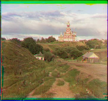
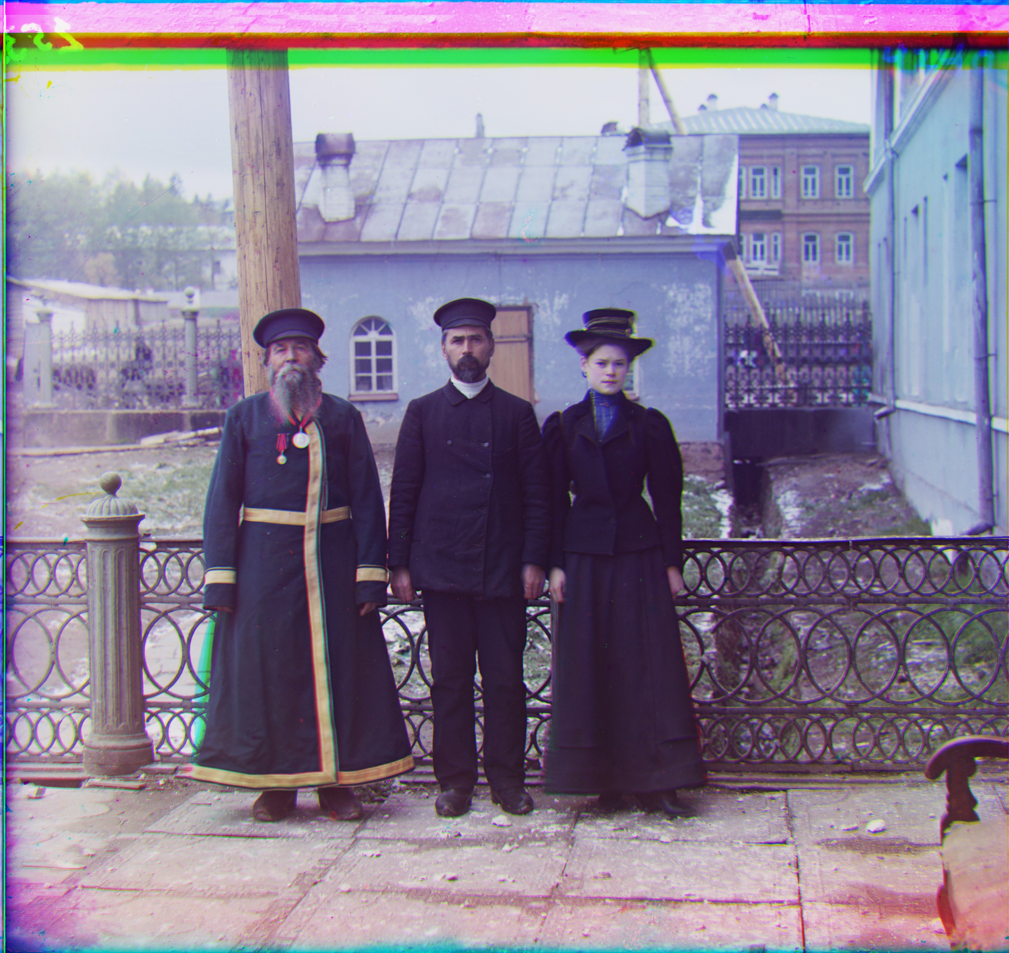
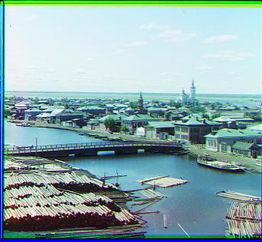
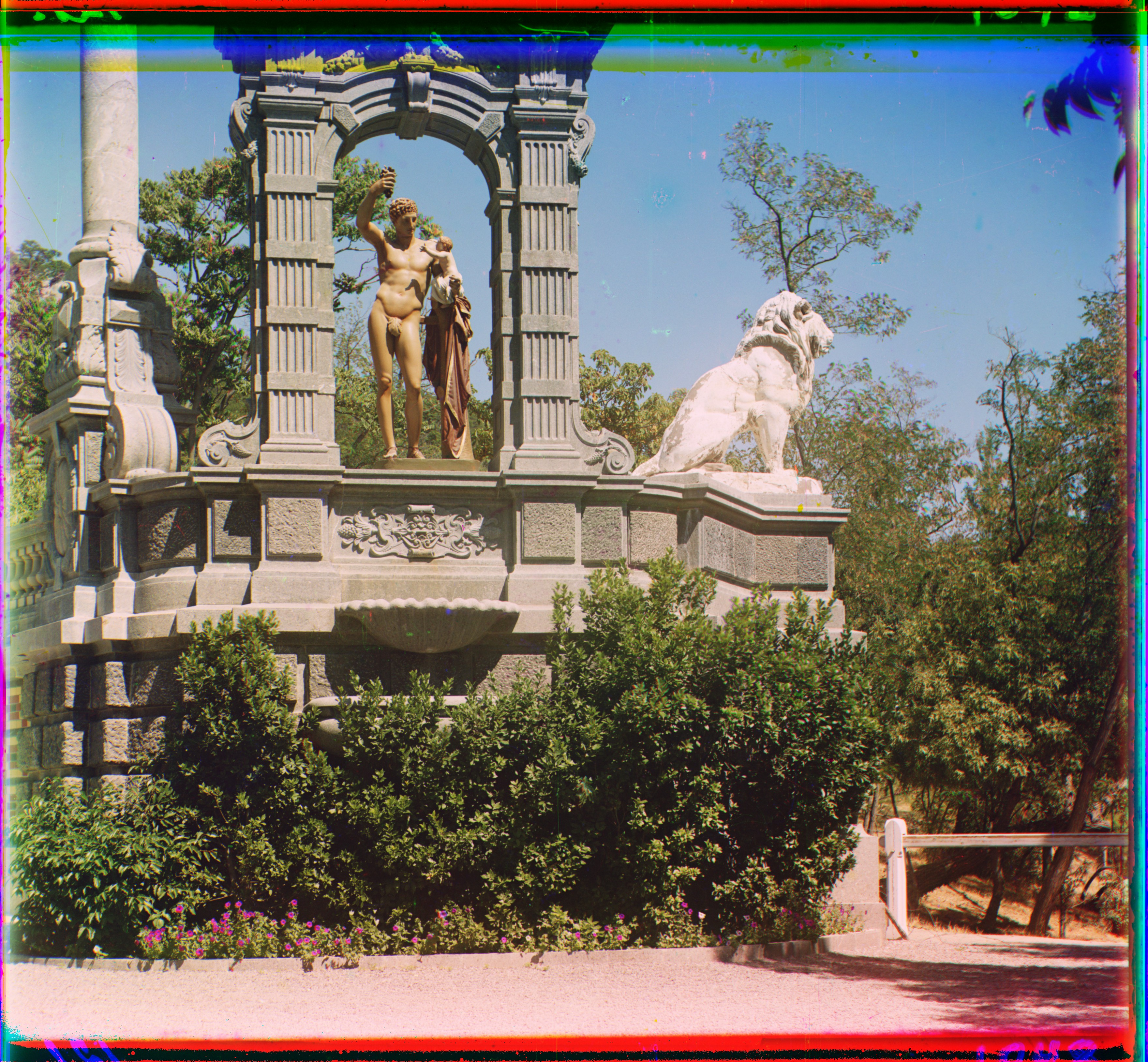
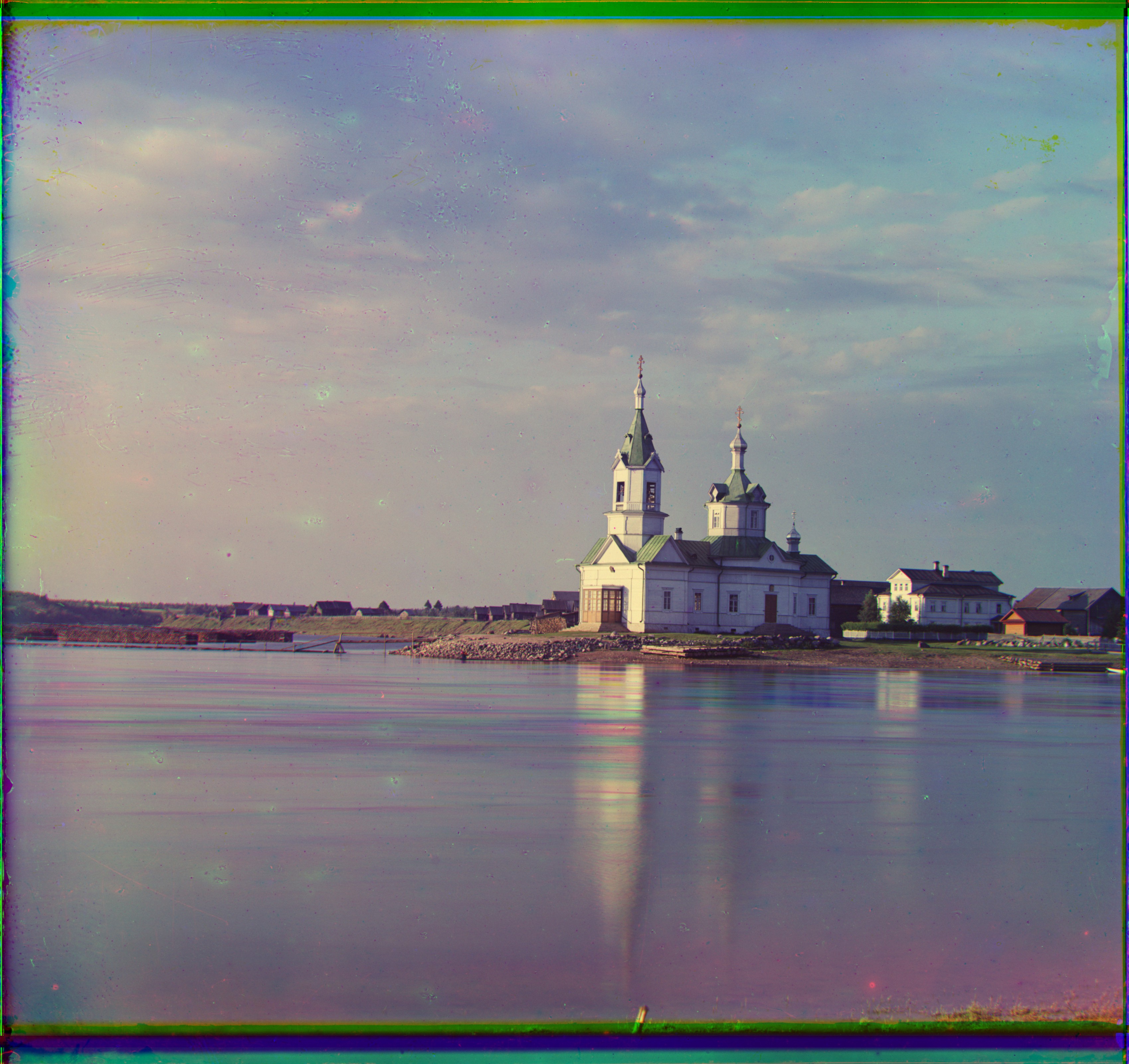
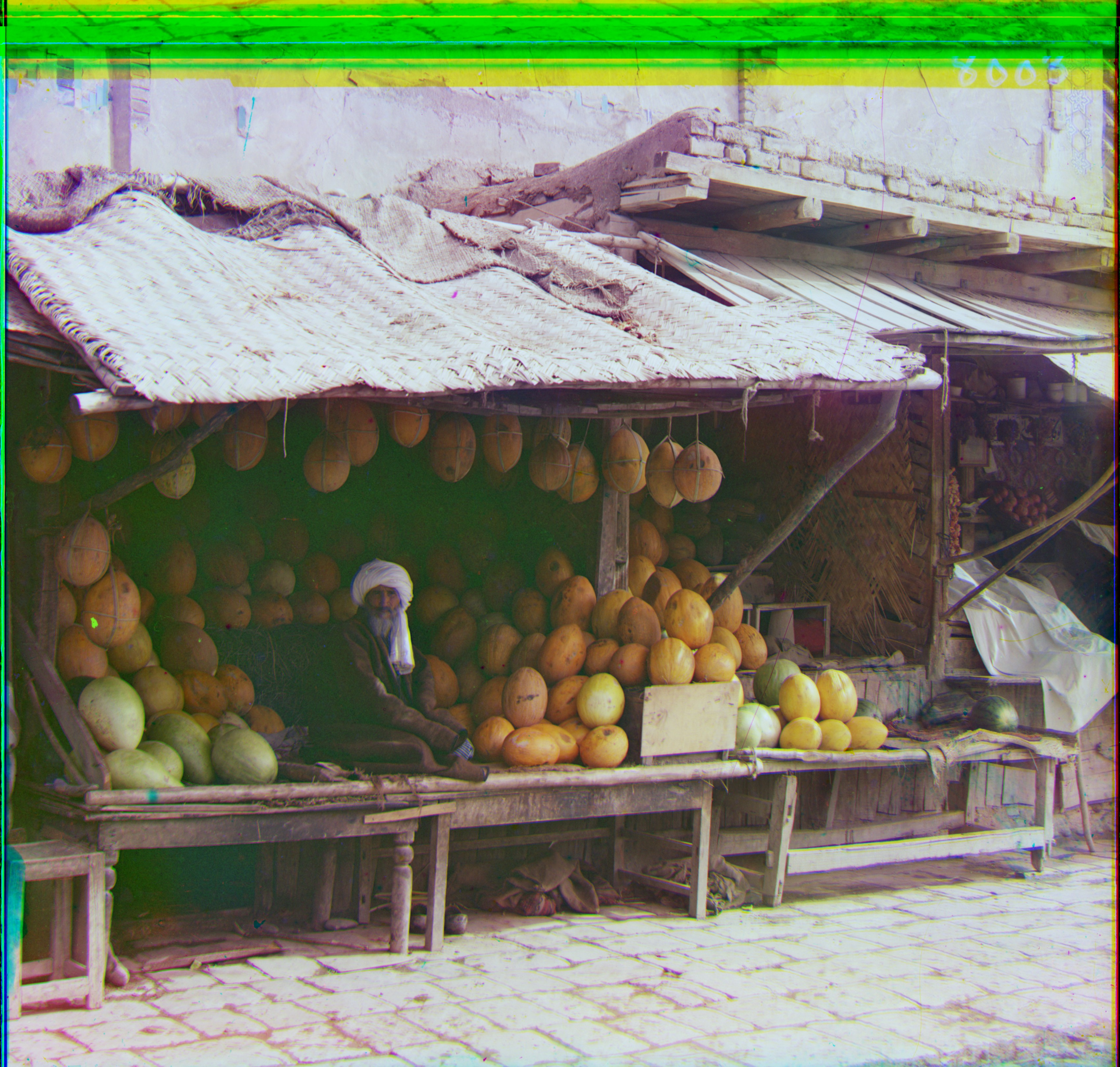
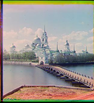
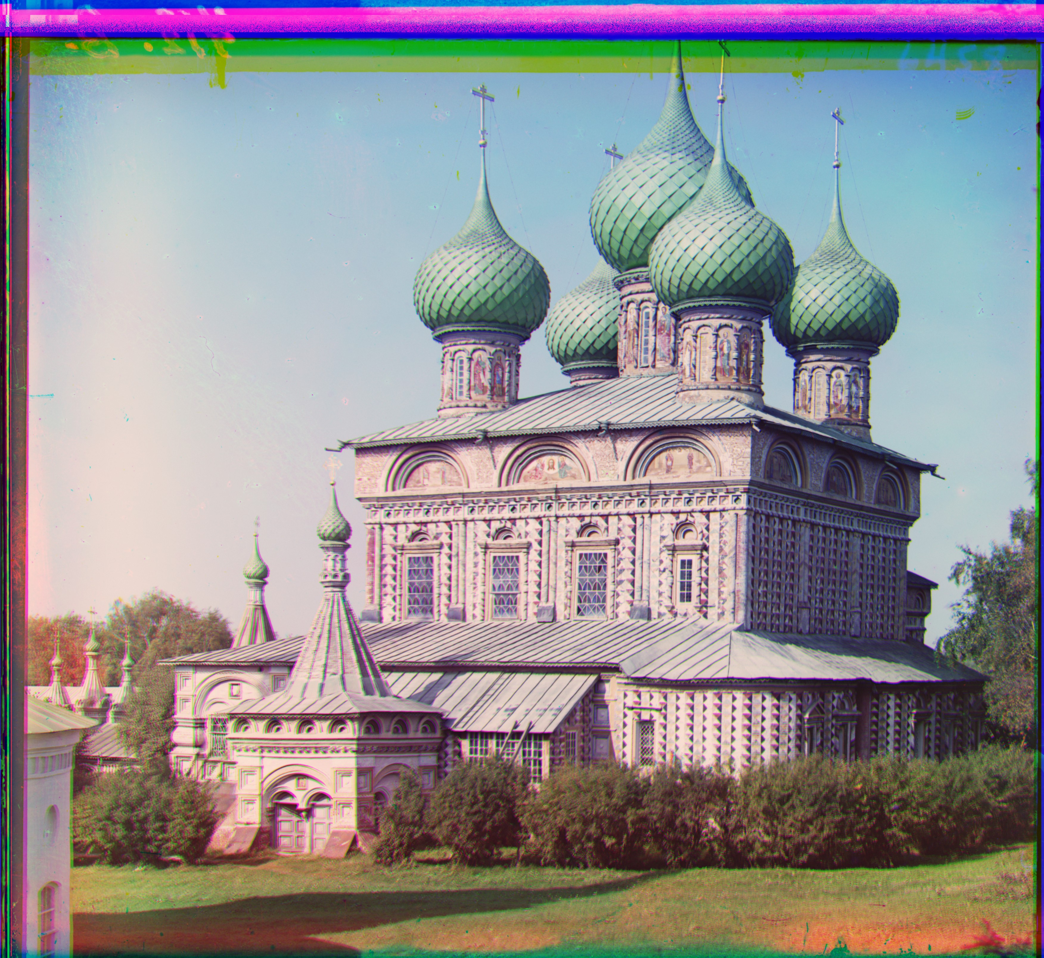
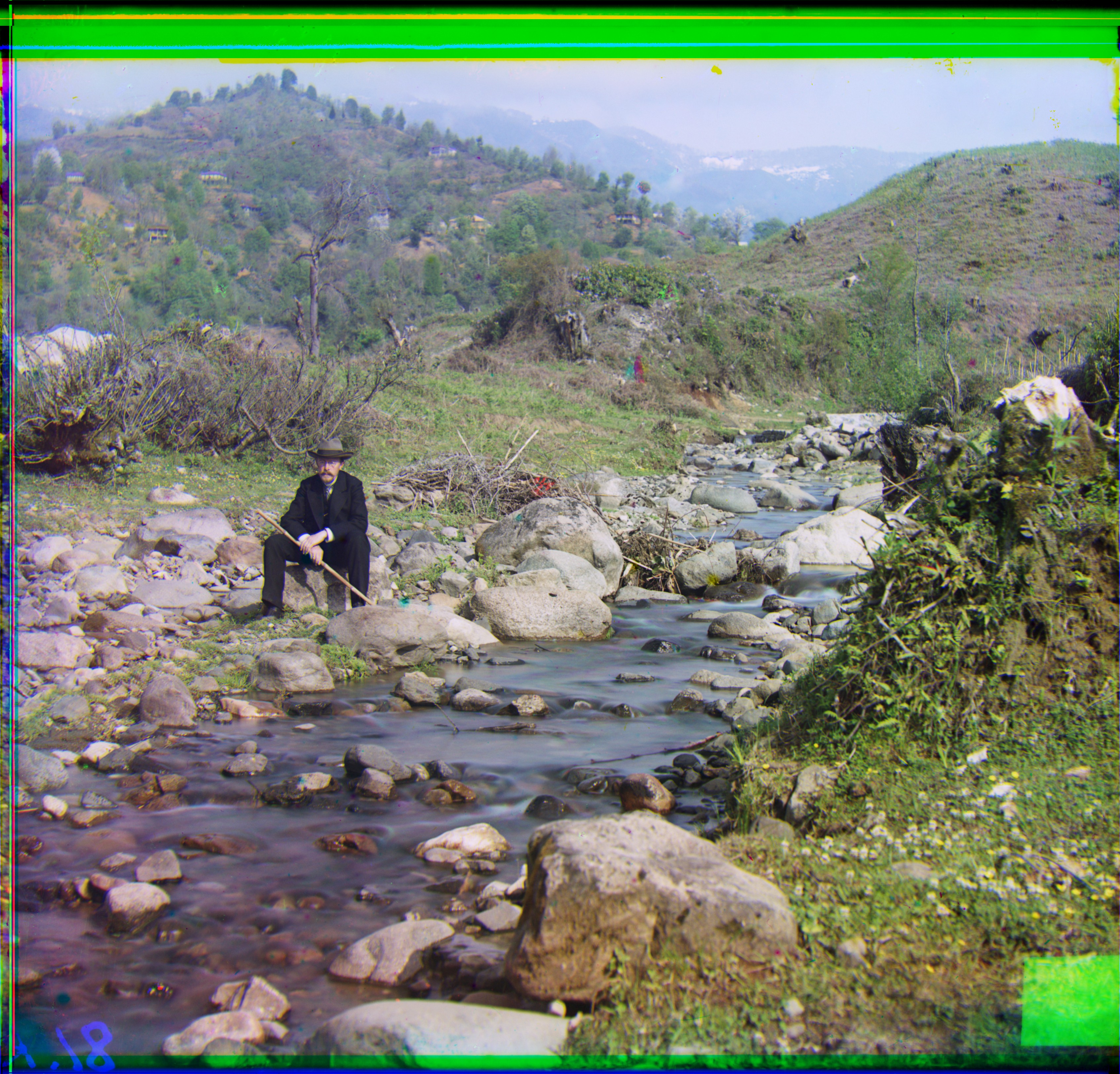
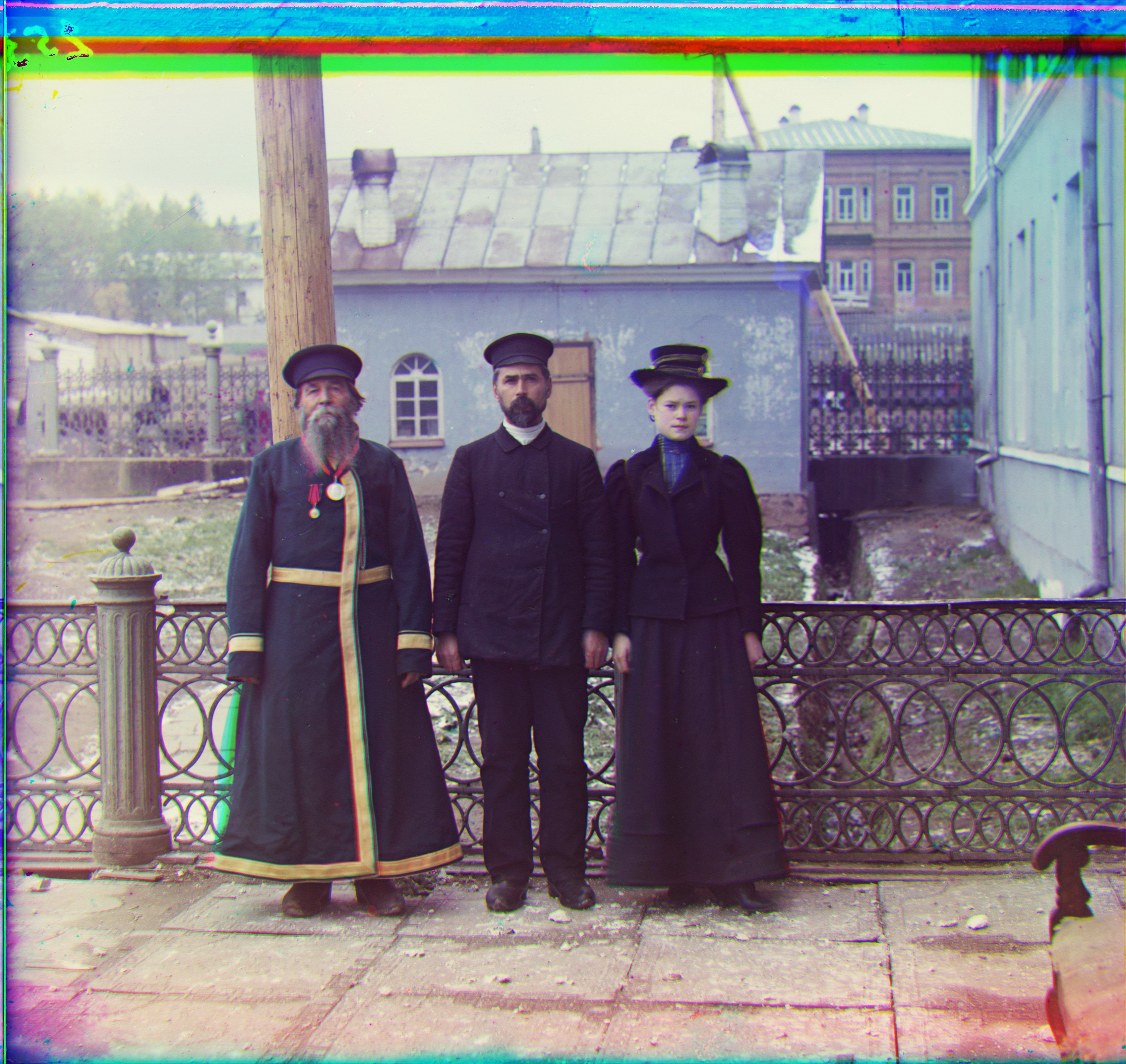
Interim Result Gallery
Rshift: (41, 106) |
Rshift: (3, 12) |
Rshift: (-4, 58) |
Rshift: (14, 123) |
Rshift: (23, 90) |

Rshift: (12, 118) |
Rshift: (13, 177) |
Rshift: (2, 3) |
Rshift: (37, 108) |

Rshift: (-27, 140) |
Rshift: (37, 175) |
Rshift: (11, 111) |
Rshift: (3, 7) |

Rshift: (31, 85) |
Figure 3: My interim results with multi-layer matching.
The G & R Value below the image are shift values of green & red channel.
Post-Processing on Images
Auto White-Balancing
In this project, we implement the gray world algorithm, which is a classic auto white balance algorithm that estimates the illuminant of an image by assuming that the average color of the world is gray. The algorithm is based on the idea that the average reflectance of surfaces in the world is achromatic, or gray.
Remark: when calculating the mean values, the outer 10% of the image border is excluded to avoid potential biases (since the image itself is damaged).
Auto Contrasting
This is a straightforward algorithm. We select the minimum & maximum value \(\min, \max\) among the three channels and remap the entire image to \([0, 255]\) accordingly. It’s important to note that we do not apply auto-contrasting separately to each channel, as doing so would disrupt the white balance established in section 2.1.
Ablation Study
|
|
|
Figure 4: Auto-contrasting & white-balancing (left: off; right: on)
|
|
|
Figure 5: Auto-contrasting & white-balancing (top: off; bottom: on)
In comparison, the images on the left are overly blue, green, or red. The auto-contrasting and white-balancing algorithms have made slight adjustments to improve their appearance.
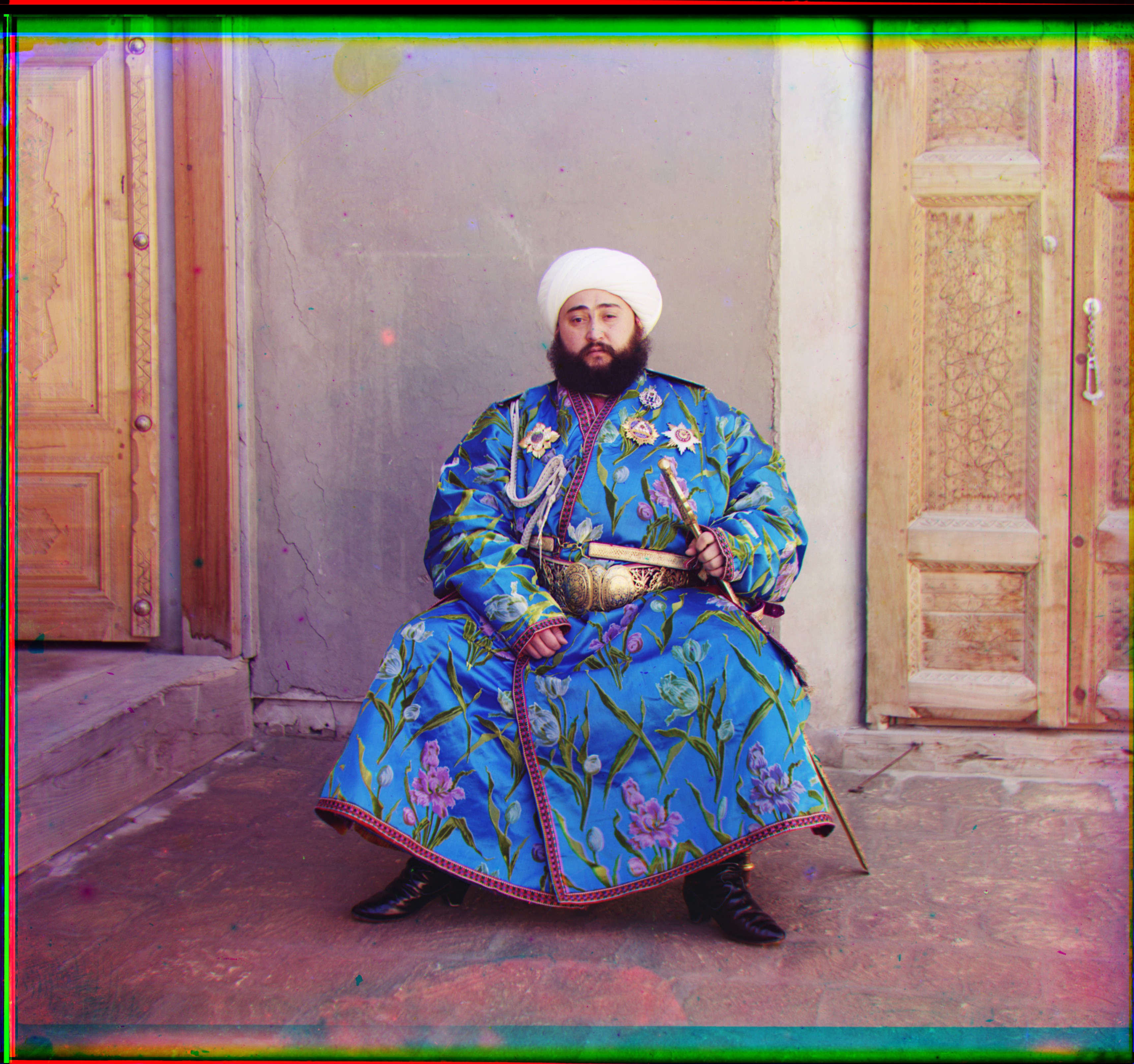
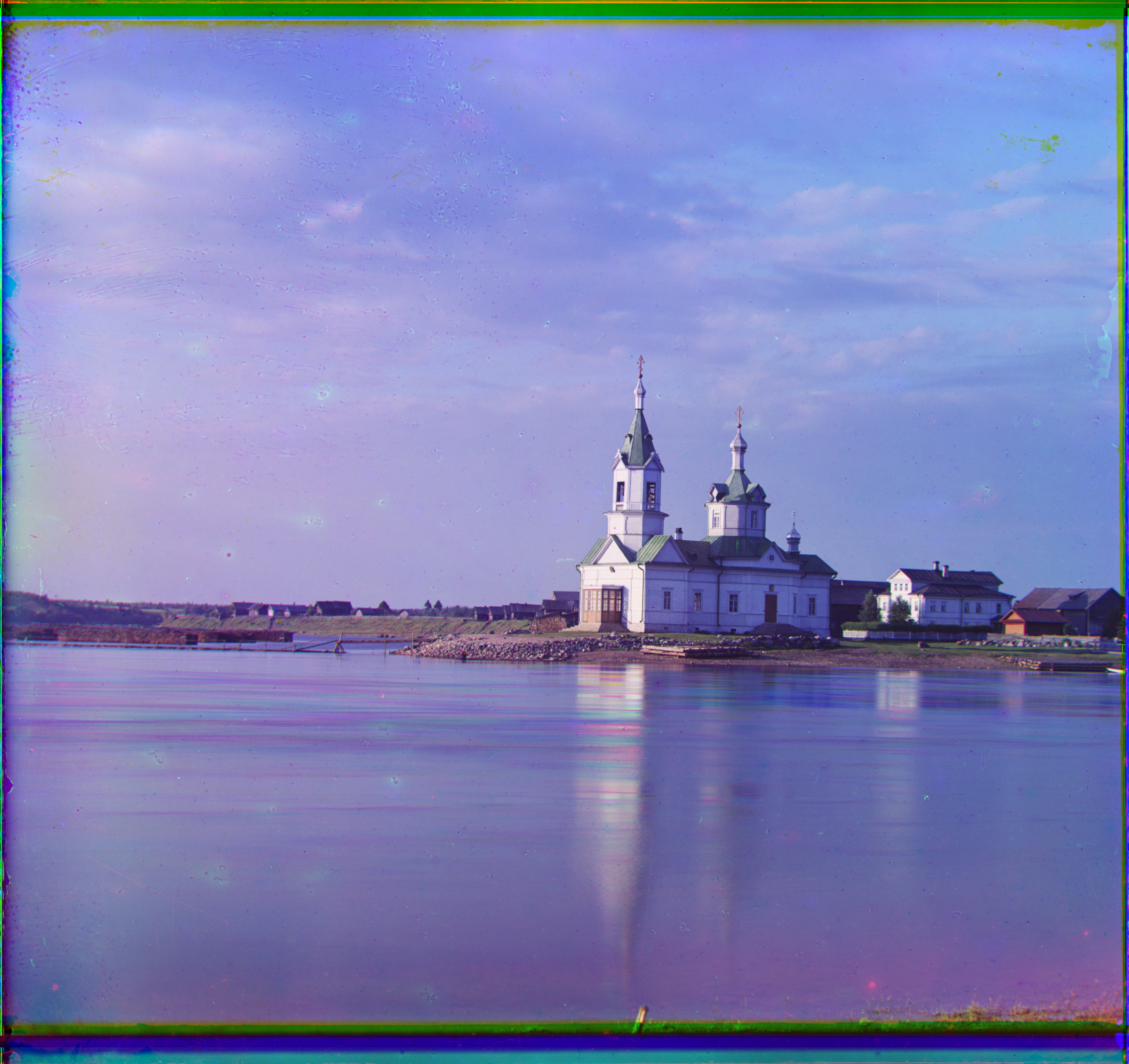
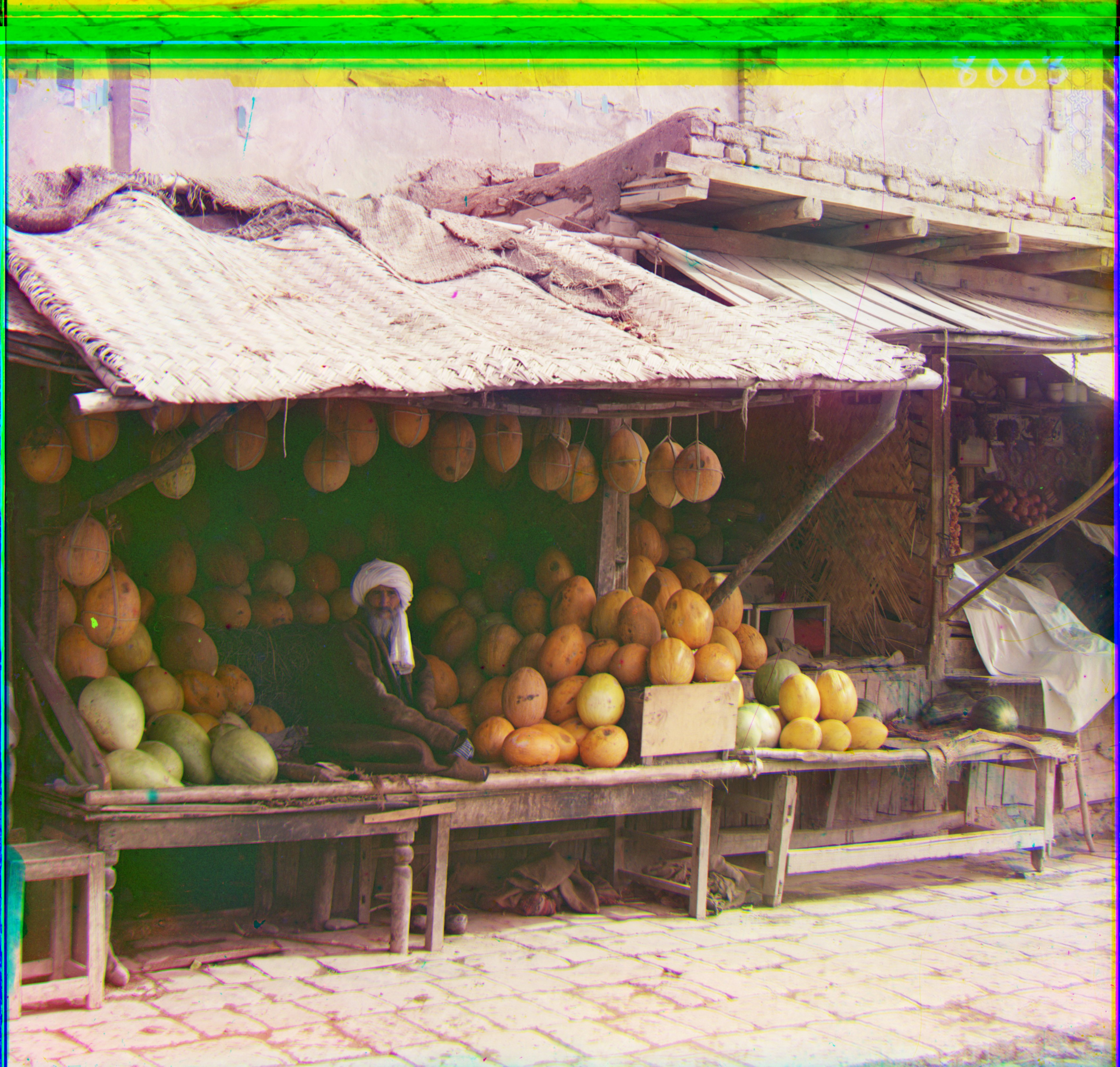
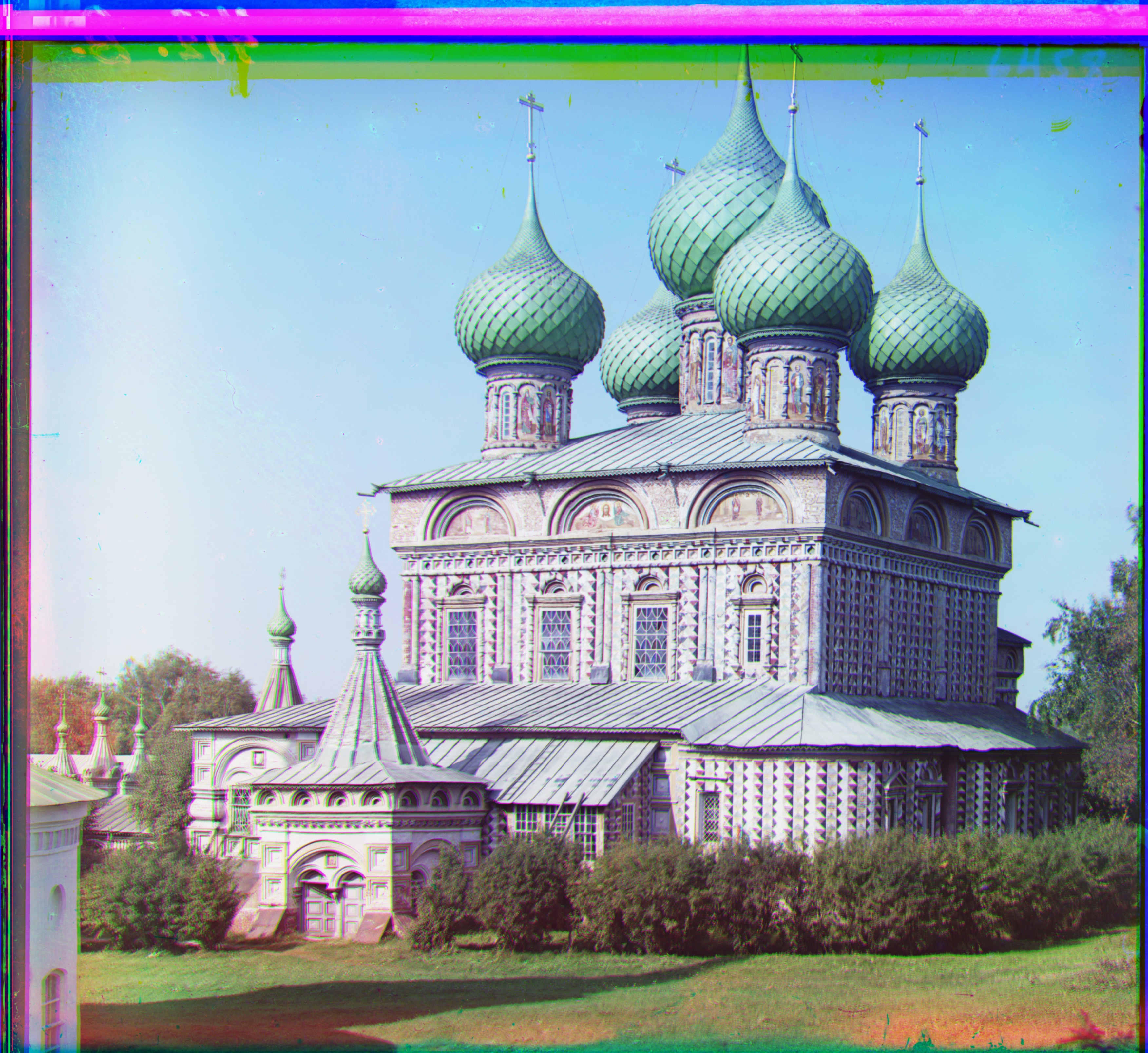
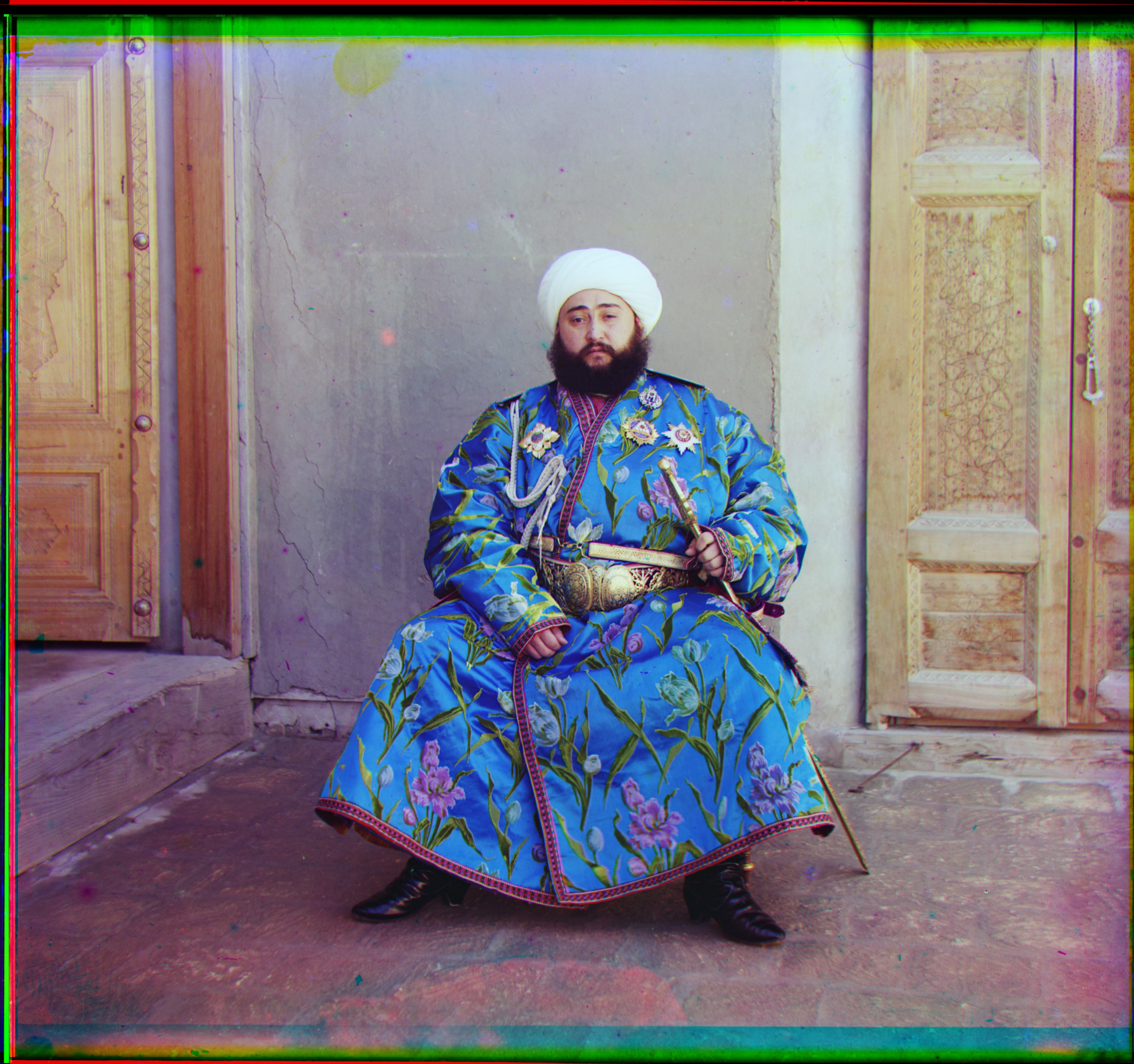
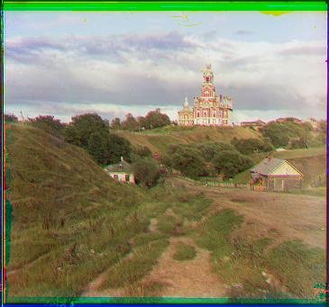
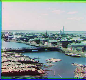
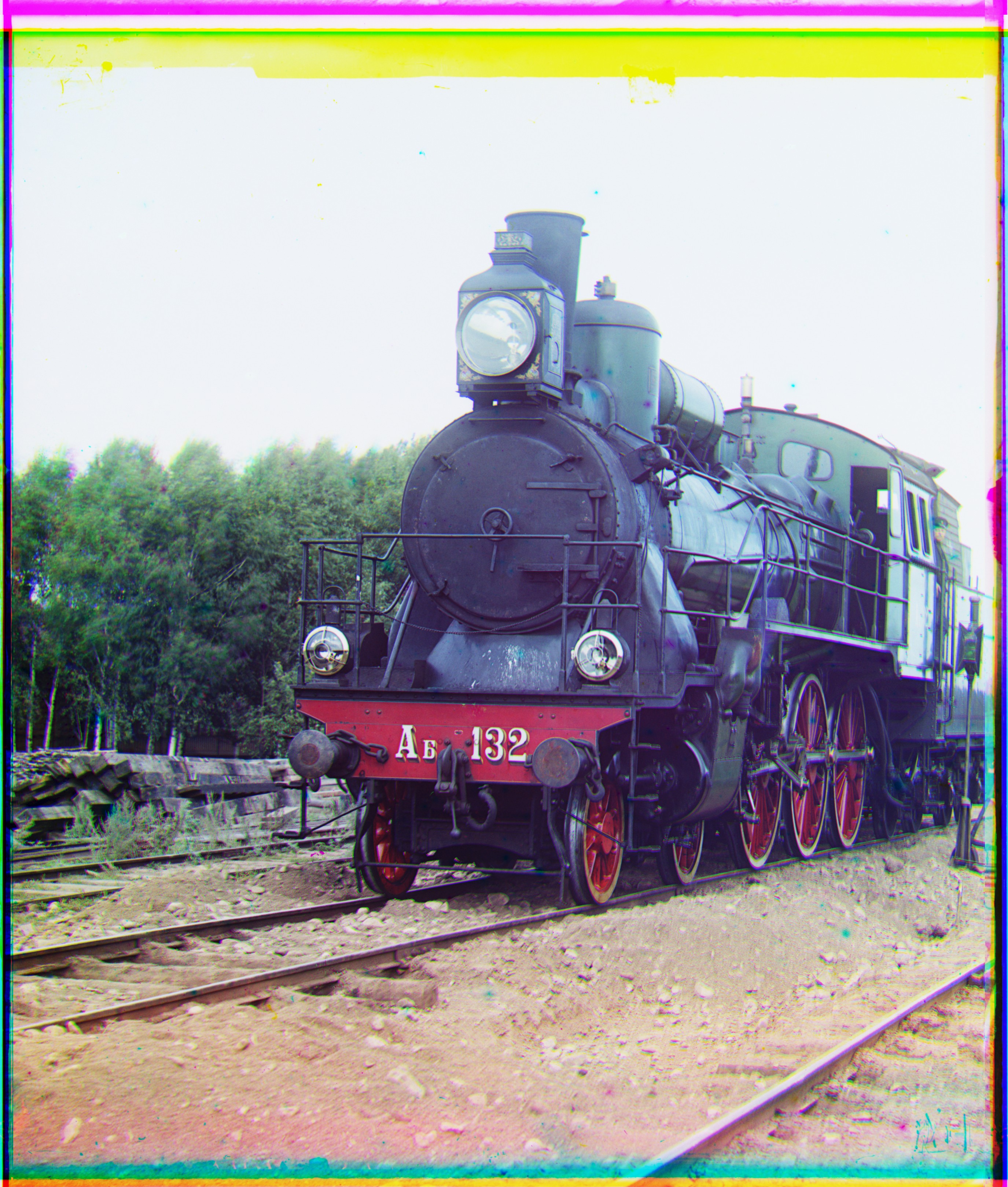
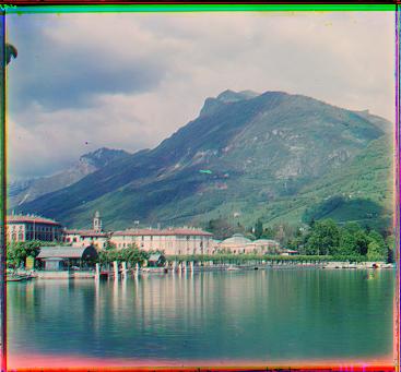
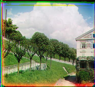
Final Results
Here are all mandatory final results.
|
|
|
|
|
|
|
|
|
|
|
|
|
|
|
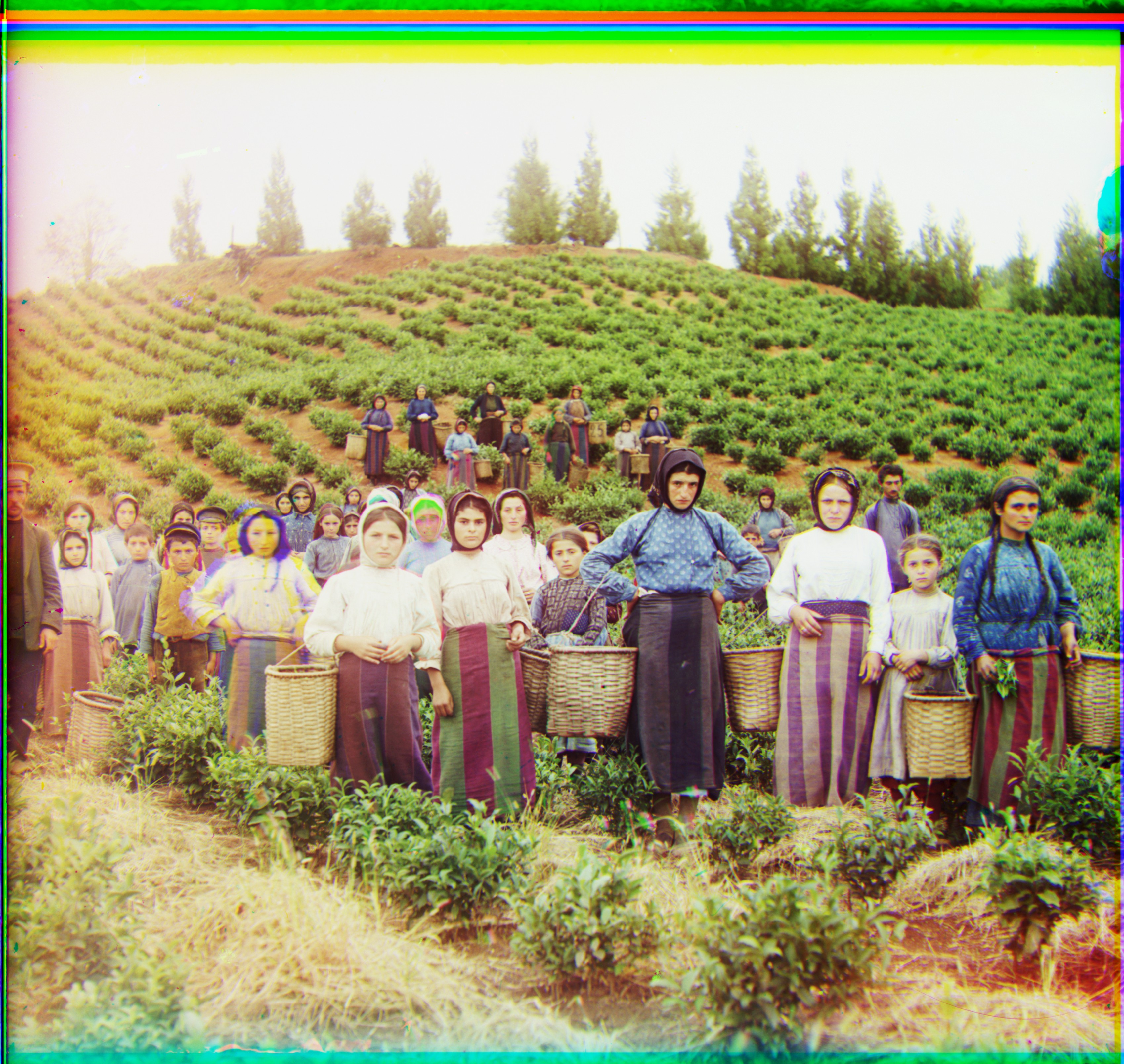
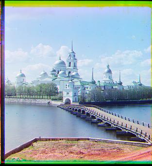
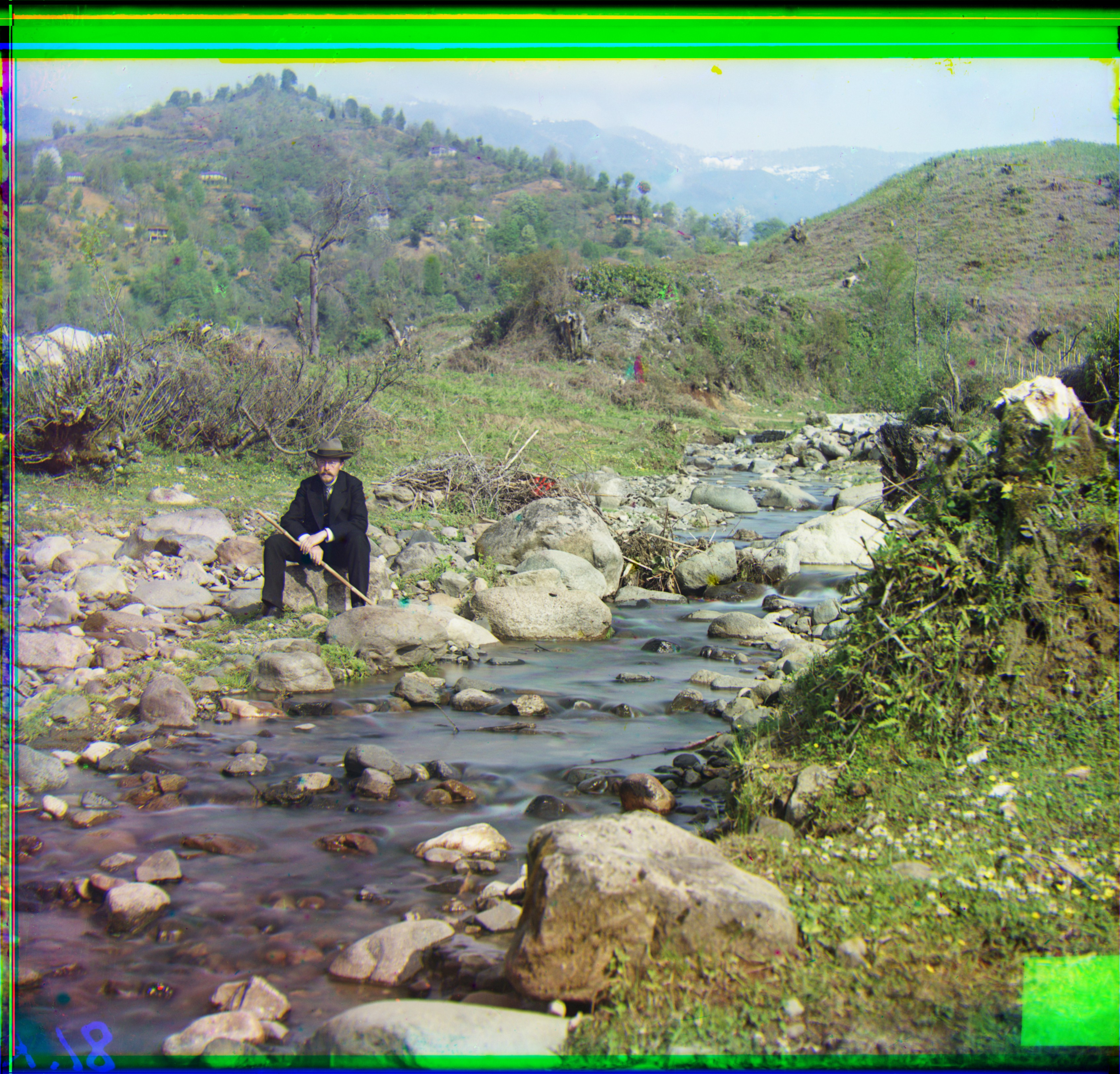
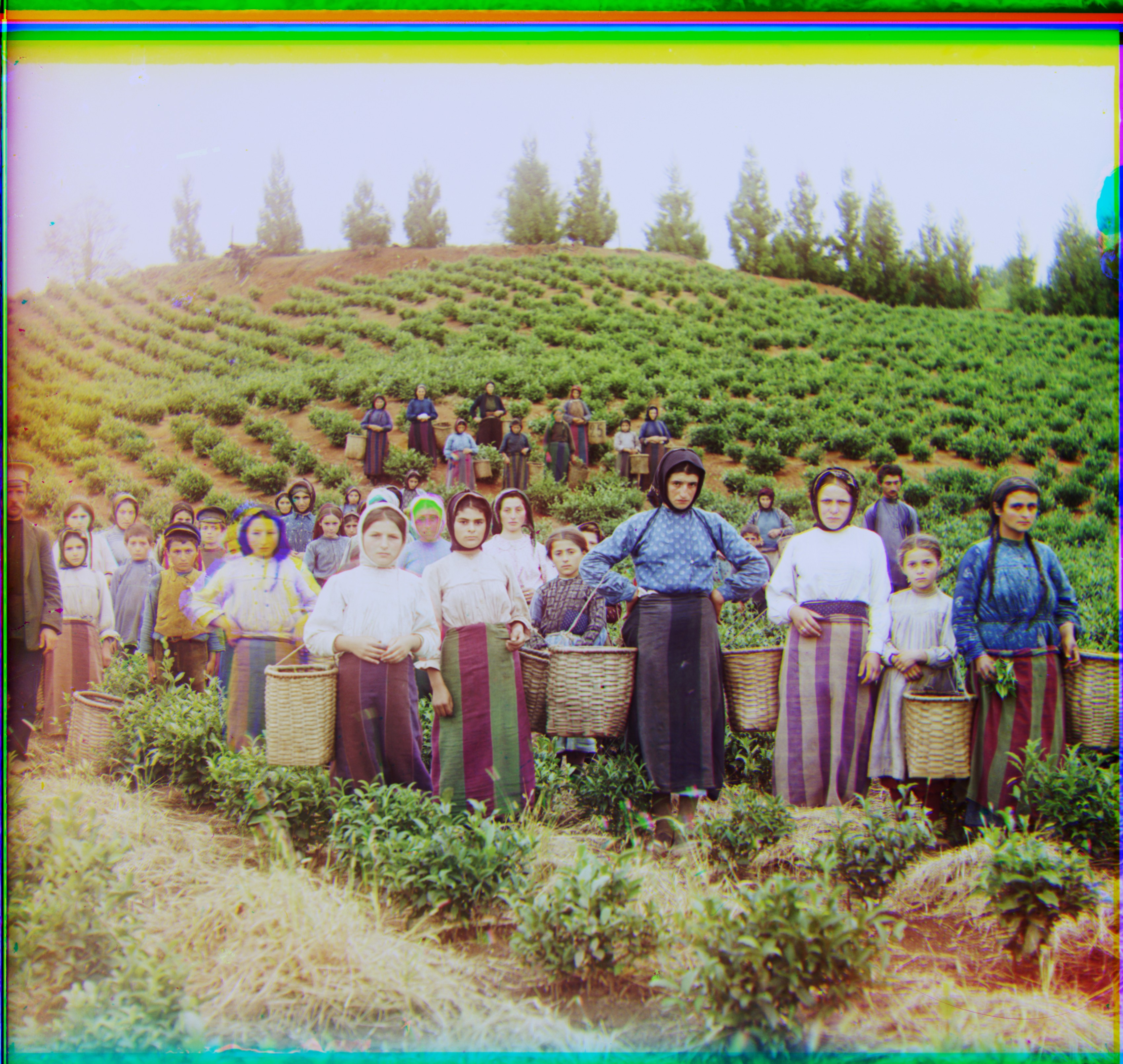
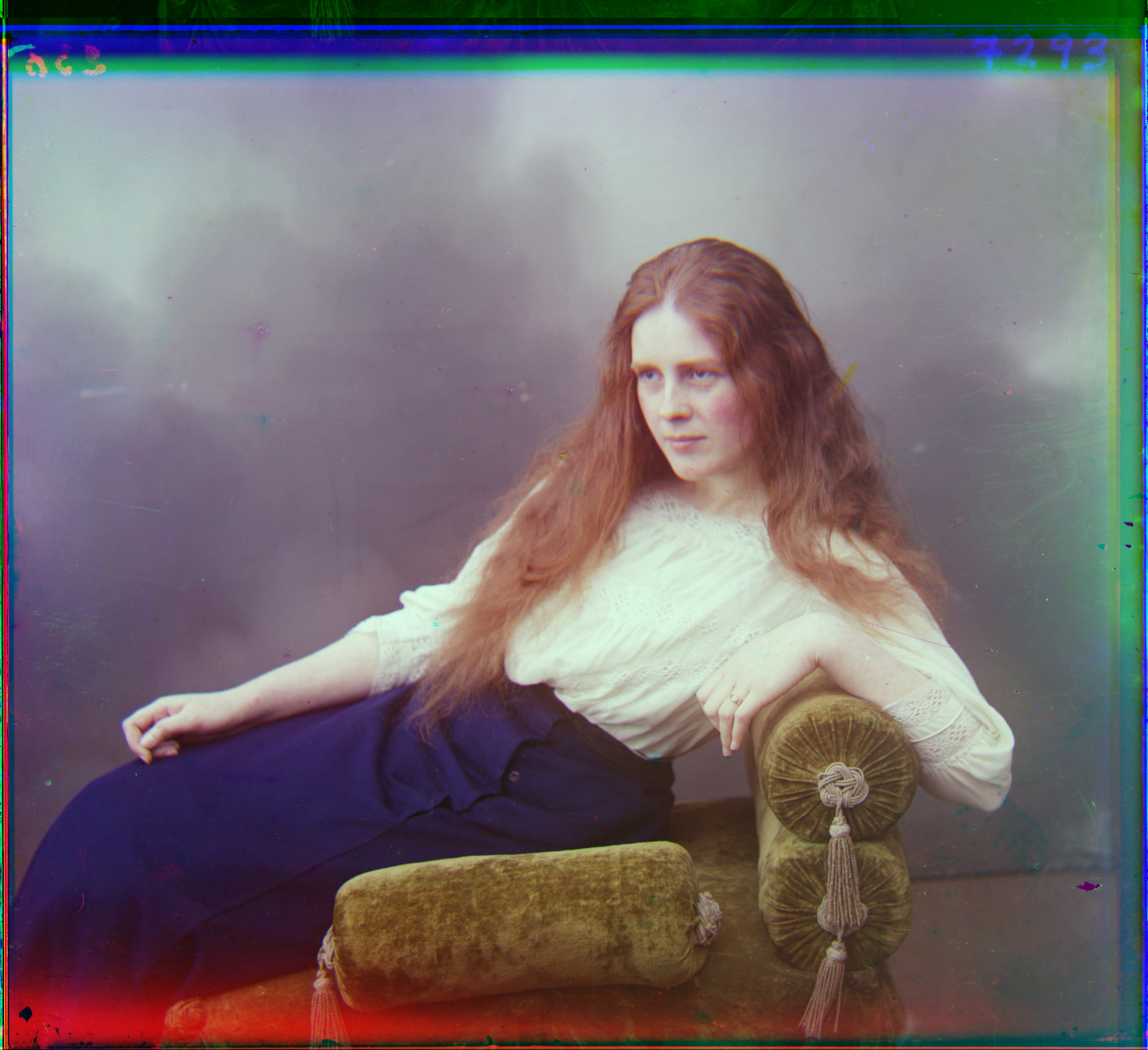
More Results
Here are some results that I appreciate!
|
|