
Project Overview
- UC Berkeley CV Project 5a: Fun with Diffusion Models
- Iterative Denoising
- Classifier Free Guidance
- Img2Img Translation via SDEdit
- Visual Anagrams
- Image Hybriding via Factorized Diffusion
- UC Berkeley CV Project 5b: Implement DDPM Yourself
- Define UNet Structure
- Train with noised dataset
Part A: Fun with Diffusion Models
Remark: For all subsequent sections in part A, we use
20040805as our seed.We will call
seed()every time before we generate pictures to make all the results reproducible.
Setup
First, we setup the DeepFloyd IF diffusion model.
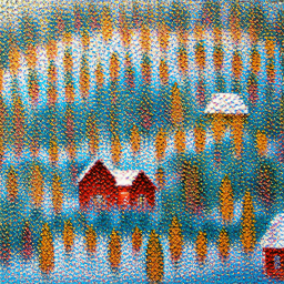
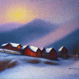
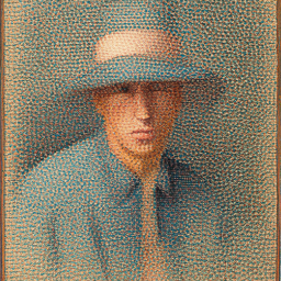
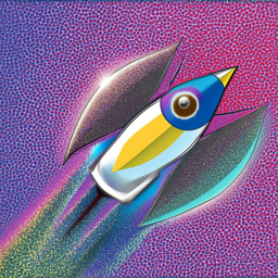
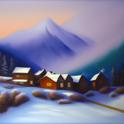
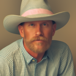
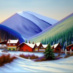
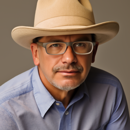
Here are some example images generated by DeepFloydIF, using 3
different text prompts and different num_inference_steps.
It can be read from the results that with higher num_inference_steps the
image is more complete.
|
Inference step Text prompt |
An oil painting of a snowy mountain village |
A man wearing a hat | A rocket ship |
|---|---|---|---|
| Step=2 |
|
|
|
| Step=4 |
|
|
|
| Step=6 |
|
|
|
| Step=8 |
|
|
|
| Step=12 |
|
|

|
| Step=16 |
|
|

|
Forward Process
A key part of diffusion is the forward process, which takes a clean image and adds noise to it. In this part, we will write a function to implement this. The forward process is defined by: \[ q(x_t|x_0) = N(x_t; \sqrt{\bar{\alpha}_t}x_0, (1 - \bar{\alpha}_t)\mathbf{I}) \] Which is equivalent to computing: \[ x_t = \sqrt{\bar{\alpha}_t}x_0 + \sqrt{1 - \bar{\alpha}_t}\epsilon \quad \text{where} \quad \epsilon \sim N(0, 1) \] That is, given a clean image \(x_0\), we get a noisy image \(x_t\) at timestep \(t\) by sampling from a Gaussian with mean \(\sqrt{\bar{a_t}}x_0\) and variance \(\sqrt{1-\bar{a_t}}\).
Here is an example showing the process of adding noise to a single image.
| t=000 | t=125 | t=250 | t=375 | t=500 | t=625 | t=750 | t=875 | |
|---|---|---|---|---|---|---|---|---|
|
Noisy Image |

|

|

|

|

|

|

|

|
Classical Denoising
Let's try to denoise these images using classical methods. Again, take noisy images, but use Gaussian blur filtering to try to remove the noise. Getting good results should be quite difficult, if not impossible.
| t=000 | t=125 | t=250 | t=375 | t=500 | t=625 | t=750 | t=875 | |
|---|---|---|---|---|---|---|---|---|
|
Noisy Image |
|
|
|
|
|
|
|
|
| Blurr Image |

|

|

|

|

|

|

|

|
One-Step Denoising
Now, we'll use a pretrained diffusion model to denoise. The actual
denoiser is stage_1.unet. This is a UNet that has already
been trained on a very, very large dataset of \((x_0,x_t)\) pairs of images. We can use it
to recover Gaussian noise from the image. Then, we can remove this noise
to recover (something close to) the original image. The denoising
process is defined as: \[
x_0 = \frac{1}{\sqrt{\bar{\alpha}_t}} \left( x_t - \sqrt{1 -
\bar{\alpha}_t} \epsilon \right) \quad \text{where} \quad \epsilon \sim
N(0, 1)
\] Note1: This UNet is conditioned on the amount of Gaussian
noise by taking timestep t as additional input.
Note2: Because this diffusion model was trained with text
conditioning, we also need a text prompt embedding. We use the prompt
embedding "a high quality photo" generated by T5
Text Encoder.
| t=000 | t=125 | t=250 | t=375 | t=500 | t=625 | t=750 | t=875 | |
|---|---|---|---|---|---|---|---|---|
|
Noisy Image |
|
|
|
|
|
|
|
|
|
One-step Denoised Image |

|

|

|

|

|

|

|

|
Iterative Denoising
In the previous section, we can see that the denoising UNet does a much better job of projecting the image onto the natural image manifold, but it does get worse as you add more noise. This makes sense, as the problem is much harder with more noise.
But diffusion models are designed to denoise iteratively. In this part we will implement this.
In theory, we could start with noise \(x_{1000}\) at timestep \(T=1000\), denoise for one step to get an estimate of \(x_{999}\), and carry on until we get \(x_0\). But this would require running the diffusion model 1000 times, which is quite slow (and costs $$$).
It turns out, we can actually speed things up by skipping steps. The rationale for why this is possible is due to a connection with differential equations. Check this excellent article.
To skip steps we can create a new list of timesteps that we'll call
strided_timesteps, which does just this.
strided_timesteps will correspond to the noisiest image
(and thus the largest t) and strided_timesteps[-1] will
correspond to a clean image. One simple way of constructing this list is
by introducing a regular stride step (e.g. stride of 30 works well).
On the ith denoising step we are at t=
strided_timesteps[i], and want to get to t′=
strided_timesteps[i+1] (from more noisy to less noisy). To
actually do this, we have the following formula:
The formula is given as:
\[ x_{t'} = \frac{\sqrt{\bar{\alpha}_{t'} / \beta_t}}{1 - \bar{\alpha}_t} x_0 + \frac{\sqrt{\alpha_t}(1 - \bar{\alpha}_{t'})}{1 - \bar{\alpha}_t} x_t + v_\sigma \]
Where:
- \(x_t\) is image at timestep \(t\).
- \(x_{t'}\) is noisy image at timestep \(t'\) where \(t' < t\) (less noisy).
- \(\bar{\alpha}_t\) is defined by
alphas_cumprod, as explained above. - \(\alpha_t = \frac{\bar{\alpha}_t}{\bar{\alpha}_{t-1}}\).
- \(\beta_t = 1 - \alpha_t\).
- \(x_0\) is our current estimate of the clean image using equation A.2 just like in section 1.3.
The \(v_\sigma\) is random noise, which in the case of DeepFloyd is also predicted.
Here is an example result, showing the process of strided iterative denoising.
| t=660 | t=510 | t=360 | t=210 | t=60 | t=0 | |
|---|---|---|---|---|---|---|
|
Noisy Image |

|

|

|

|

|

|
For your comparison, here is a summary of all denoising results, using all aforementioned algorithms.
| Original Image | Gaus Blur Denoised | One-Step Denoised | Iterative Denoised |
|---|---|---|---|
|
|

|

|
|
Diffusion Model Sampling
In the previous part, we use the diffusion model to denoise an image.
Another thing we can do with the iterative_denoise function
is to generate images from scratch. We can do this by setting
i_start = 0 and passing in random noise. This effectively
denoises pure noise, and we sample 5 results of
"a high quality photo" from pure noise.
| Sample 1 | Sample 2 | Sample 3 | Sample 4 | Sample 5 |
|---|---|---|---|---|

|

|

|

|

|
Classifier-Free Guidance (CFG)
You may have noticed that the generated images in the prior section are not very good, and some are completely non-sensical. In order to greatly improve image quality (at the expense of image diversity), we can use a technicque called Classifier-Free Guidance.
In CFG, we compute both a conditional and an unconditional noise estimate. We denote these \(\epsilon_c\) and \(\epsilon_u\). Then, we let our new noise estimate be \[ \epsilon = \epsilon_u + \lambda(\epsilon_c-\epsilon_u) \] where \(\lambda\) controls the strength of CFG. Notice that for \(\lambda=0\), we get an unconditional noise estimate, and for \(\lambda=1\) we get the conditional noise estimate. The magic happens when \(\lambda>1\). In this case, we get much higher quality images. Why this happens is still up to vigorous debate. For more information on CFG, you can check out this blog post.
Disclaimer: Before, we used
"a high quality photo" as a "null" condition. Now, we will
use the actual "" null prompt for unconditional guidance
for CFG and use "a high quality photo" for conditional
generation.
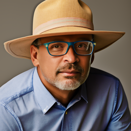
| Sample 1 | Sample 2 | Sample 3 | Sample 4 | Sample 5 |
|---|---|---|---|---|

|

|

|

|

|
Image-to-image Translation
Previously, we take a real image, add noise to it, and then denoise. This effectively allows us to make edits to existing images. The more noise we add, the larger the edit will be. This works because in order to denoise an image, the diffusion model must to some extent "hallucinate" new things -- the model has to be "creative."
Here, we're going to take the original test image, noise it somehow, and force it back onto the image manifold without any conditioning. Effectively, we're going to get an image that is similar to the test image (with a low-enough noise level), or an image that is far from the test image (with a high-enough noise level). This follows the SDEdit algorithm.
We show some results here.
Unconditioned Img2Img
| Original Image | SDEdit 20 | SDEdit 10 | SDEdit 07 | SDEdit 05 | SDEdit 03 | SDEdit 01 |
|---|---|---|---|---|---|---|

|

|

|

|

|

|

|

|

|

|

|

|

|

|

|

|

|

|

|

|

|
Hand-Drawn Img Editing
| Original Image | SDEdit 20 | SDEdit 10 | SDEdit 07 | SDEdit 05 | SDEdit 03 | SDEdit 01 |
|---|---|---|---|---|---|---|

|

|

|

|

|

|

|

|

|

|

|

|

|

|

|

|

|

|

|

|

|
Text-Conditioned Img2Img
We will do the same thing as SDEdit, but guide the projection with a
text prompt. This is no longer pure "projection to the natural image
manifold" but also adds control using language. This is simply a matter
of changing the prompt from "a high quality photo" to any
other prompts.
| Original Image | SDEdit 20 | SDEdit 10 | SDEdit 07 | SDEdit 05 | SDEdit 03 | SDEdit 01 |
|---|---|---|---|---|---|---|

|

|

|

|

|

|

|
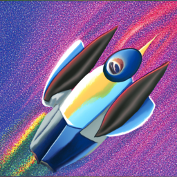
| Text Prompt: "a rocket ship" | ||||||

|

|

|

|

|

|

|
| Text Prompt: "a photo of a dog" | ||||||

|

|

|

|

|

|

|
| Text Prompt: "a man wearing a hat" | ||||||
In-Painting
We can use the same procedure to implement inpainting (following the RePaint paper). That is, given an image \(x_{\text{orig}}\) and a binary mask \(\mathbf{m}\), we can create a new image that has the same content where \(\mathbf{m} = 0\), but new content wherever \(\mathbf{m} = 1\).
To do this, we can run the diffusion denoising loop. But at every step, after obtaining \(x_t\), we "force" \(x_t\) to have the same pixels as \(x_{\text{orig}}\) where \(\mathbf{m} = 0\), i.e.:
\[ x_t \leftarrow \mathbf{m} x_t + (1 - \mathbf{m}) \text{forward}(x_{\text{orig}}, t) \]
Essentially, we leave everything inside the edit mask alone, but we replace everything outside the edit mask with our original image -- with the correct amount of noise added for timestep \(t\).
| Original Image | Mask | Hole to Fill | Inpainted Image |
|---|---|---|---|

|

|

|

|

|

|

|

|

|

|

|

|
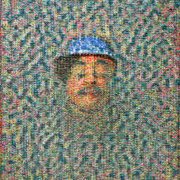
Visual Anagrams
In this part, we are finally ready to implement Visual Anagrams and create optical illusions with diffusion models. In this part, we will create an image that looks like "an oil painting of an old man", but when flipped upside down will reveal "an oil painting of people around a campfire".
To do this, we will denoise an image \(x_t\) at step \(t\) normally with the prompt "an oil painting of an old man", to obtain noise estimate \(\epsilon_1\). But at the same time, we will flip \(x_t\) upside down, and denoise with the prompt "an oil painting of people around a campfire", to get noise estimate \(\epsilon_2\). We can flip \(\epsilon_2\) back, to make it right-side up, and average the two noise estimates. We can then perform a reverse/denoising diffusion step with the averaged noise estimate.
The full algorithm will be:
\[ \epsilon_1 = \text{UNet}(x_t, t, p_1) \] \[ \epsilon_2 = \text{flip}(\text{UNet}(\text{flip}(x_t), t, p_2)) \] \[ \epsilon = \frac{\epsilon_1 + \epsilon_2}{2} \]
Where UNet is the diffusion model UNet from before, \(\text{flip}(\cdot)\) is a function that flips the image, and \(p_1\) and \(p_2\) are two different text prompt embeddings. And our final noise estimate is \(\epsilon\).
Here are some example results produced.
| An oil painting of an old man | An oil painting of people around a campfire |
|---|---|

|

|
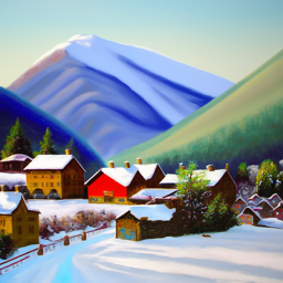
| An oil painting of a snowy mountain village | A photo of a hipster barista |

|

|
| A photo of the amalfi coast | An oil painting of a snowy mountain village |

|

|
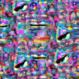
Hybrid Images
In this part, we'll implement Factorized Diffusion and create hybrid images.
In order to create hybrid images with a diffusion model, we can use a similar technique as above. We will create a composite noise estimate \(\epsilon\), by estimating the noise with two different text prompts, and then combining low frequencies from one noise estimate with high frequencies of the other. The algorithm is:
\[ \epsilon_1 = \text{UNet}(x_t, t, p_1) \] \[ \epsilon_2 = \text{UNet}(x_t, t, p_2) \] \[ \epsilon = f_{\text{lowpass}}(\epsilon_1) + f_{\text{highpass}}(\epsilon_2) \]
Where UNet is the diffusion model UNet, \(f_{\text{lowpass}}\) is a low-pass function, \(f_{\text{highpass}}\) is a high-pass function, and \(p_1\) and \(p_2\) are two different text prompt embeddings. Our final noise estimate is \(\epsilon\).
| A lithograph of a skull | A lithograph of waterfalls |
|---|---|

|
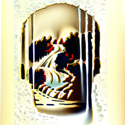
|
| A lithograph of a skull | An oil painting of a snowy mountain village |

|

|
| An oil painting of an old man | An oil painting of people around a campfire |

|

|
Part B: Training Your Own Diffusion Model!
Train a Single-Step Denoising UNet
Let's warm up by building a simple one-step denoiser. Given a noisy image \(z\), we aim to train a denoiser \(D_\theta\) such that it maps \(z\) to a clean image \(x\). To do so, we can optimize over an L2 loss:
\[ L = \mathbb{E}_{z, x} \|D_\theta(z) - x\|^2 \]
Implementing the UNet
In this project, we implement the denoiser as a UNet. It consists of a few downsampling and upsampling blocks with skip connections.
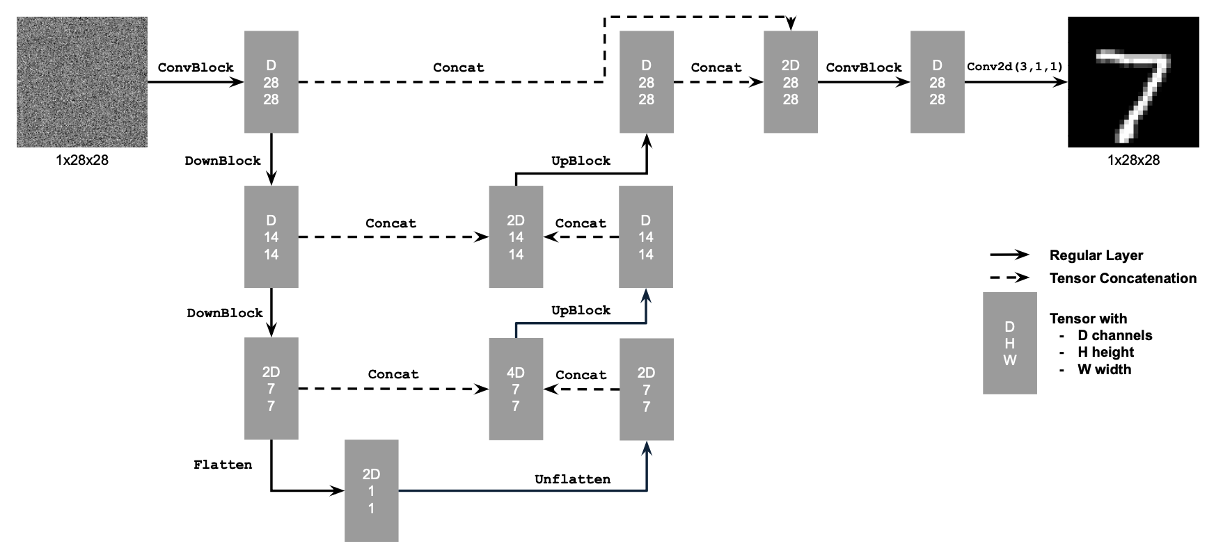
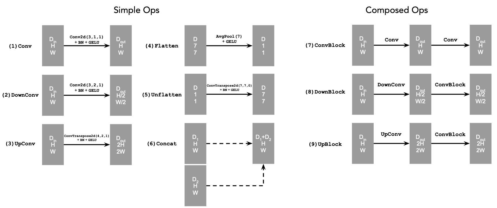
The diagram above uses a number of standard tensor operations defined as follows:
Forward Process
Recall from equation 1 that we aim to solve the following denoising problem: Given a noisy image \(z\), we aim to train a denoiser \(D_\theta\) such that it maps \(z\) to a clean image \(x\). To do so, we can optimize over an L2 loss:
\[ L = \mathbb{E}_{z, x} \|D_\theta(z) - x\|^2. \]
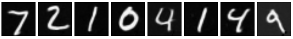
To train our denoiser, we need to generate training data pairs of \((z, x)\), where each \(x\) is a clean MNIST digit. For each training batch, we can generate \(z\) from \(x\) using the following noising process:
\[ z = x + \sigma \epsilon, \quad \text{where} \quad \epsilon \sim N(0, \mathbf{I}). \]
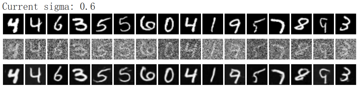
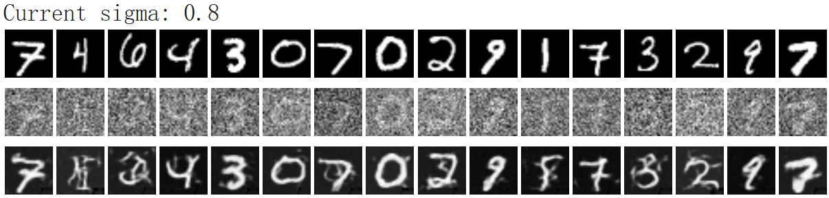
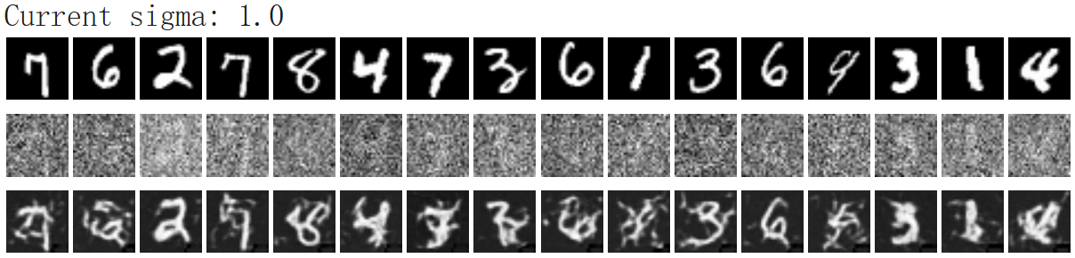
Visualize the different noising processes over \(\sigma = [0.0, 0.2, 0.4, 0.5, 0.6, 0.8, 1.0]\), assuming normalized \(x \in [0, 1]\), would get something like the following results.
Training Details
Now, we will train the model to perform denoising.
- Objective: Train a denoiser to denoise noisy image \(z\) with \(\sigma = 0.5\) applied to a clean image \(x\).
- Dataset and dataloader: Use the MNIST dataset via
torchvision.datasets.MNISTwith flags to access training and test sets. Train only on the training set. Shuffle the dataset before creating the dataloader. Recommended batch size: 256. We'll train over our dataset for 5 epochs.- You should only noise the image batches when fetched from the dataloader so that in every epoch the network will see new noised images, improving generalization.
- Model: Use the UNet architecture defined in section 1.1 with recommended hidden dimension \(D = 128\).
- Optimizer: Use Adam optimizer with learning rate of \(10^{-4}\).
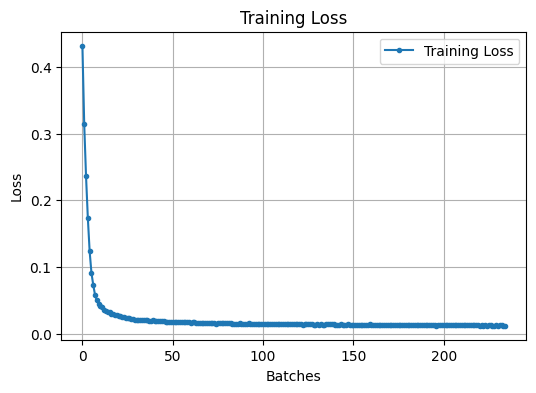
We can get some loss curve like the following graph:
Also, we can visualize after some epoch of training.
|
Original Images |
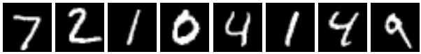
|
|
Noised Images |
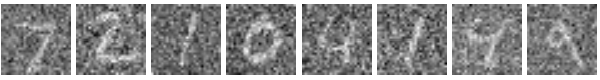
|
|
Denoised Train epoch=1 |
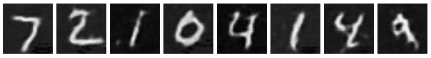
|
|
Denoised Train epoch=5 |
|
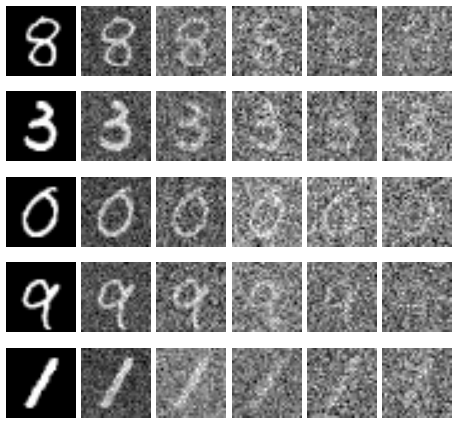
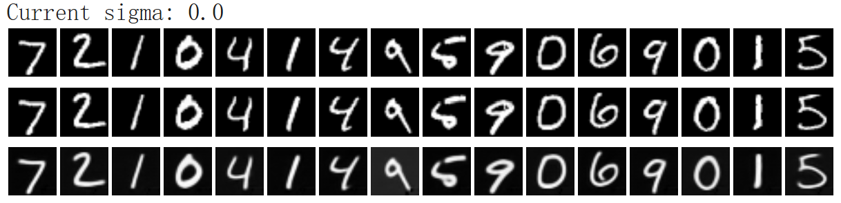
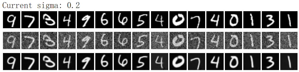
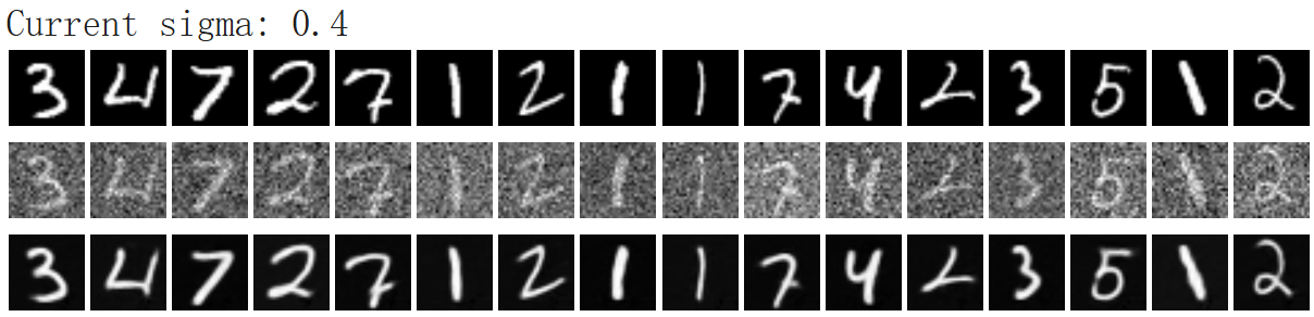
Out-of-Distribution Testing
Our denoiser was trained on MNIST digits noised with \(\sigma=0.5\). Let's see how the denoiser performs on different \(\sigma\)'s that it wasn't trained for.
Visualize the denoiser results on test set digits with varying levels of noise \(\sigma=[0.0,0.2,0.4,0.5,0.6,0.8,1.0]\).
Train a Diffusion Model
Now, we are ready for diffusion, where we will train a UNet model that can iteratively denoise an image. We will implement DDPM in this part.
Let's revisit the problem we solved previously:
\[ L = \mathbb{E}_{z, x} \|D_\theta(z) - x\|^2. \]
We will first introduce one small difference: we can change our UNet to predict the added noise \(\epsilon\) instead of the clean image \(x\). Mathematically, these are equivalent since \(x = z - \sigma \epsilon\). Therefore, we can turn equation into the following:
\[ L = \mathbb{E}_{\epsilon, z} \|\epsilon_\theta(z) - \epsilon\|^2 \]
Where \(\epsilon_\theta\) is a UNet trained to predict noise.
For diffusion, we eventually want to sample a pure noise image \(\epsilon \sim N(0, I)\) and generate a realistic image \(x\) from the noise. However, we saw in part A that one-step denoising does not yield good results. Instead, we need to iteratively denoise the image for better results.
Recall in part A that we used equation A.2 to generate noisy images \(x_t\) from \(x_0\) for some timestep \(t\) for \(t \in \{0, 1, \cdots, T\}\):
\[ x_t = \sqrt{\bar{\alpha}_t}x_0 + \sqrt{1 - \bar{\alpha}_t}\epsilon \quad \text{where} \quad \epsilon \sim N(0, 1). \]
Intuitively, when \(t = 0\) we want \(x_t\) to be the clean image \(x_0\), and for \(t = T\) we want \(x_t\) to be pure noise \(\epsilon\), and for \(t \in \{1, \cdots, T - 1\}\), \(x_t\) should be some linear combination of the two. The precise derivation of \(\bar{\alpha}_t\) is beyond the scope of this project (see DDPM paper for more details). Here, we provide you with the DDPM recipe to build a list \(\bar{\alpha}_t\) for \(t \in \{0, 1, \cdots, T\}\) utilizing lists \(\alpha\) and \(\beta\):
- Create a list \(\beta\) of length \(T\) such that \(\beta_0 = 0.0001\) and \(\beta_T = 0.02\) and all other elements \(\beta_t\) for \(t \in \{1, \cdots, T - 1\}\) are evenly spaced between the two.
- \(\alpha_t = 1 - \beta_t\)
- \(\bar{\alpha}_t = \prod_{s=1}^t \alpha_s\) is a cumulative product of \(\alpha_s\) for \(s \in \{1, \cdots, t\}\).
Because we are working with simple MNIST digits, we can afford to have a smaller \(T\) of 300 instead of the 1000 used in part A. Observe how \(\bar{\alpha}_t\) is close to 1 for small \(t\) and close to 0 for larger \(T\). \(\beta\) is known as the variance schedule; it controls the amount of noise added at each timestep.
Now, to denoise image \(x_t\), we could simply apply our UNet \(\epsilon_\theta(x_t)\) on \(x_t\) and get the noise \(\epsilon\). However, this won't work very well because the UNet is expecting the noisy image to have a noise variance \(\sigma = 0.5\) for best results, but the variance of \(x_t\) varies with \(t\). One could train \(T\) separate UNets, but it is much easier to simply condition a single UNet with timestep \(t\), giving us our final objective:
\[ L = \mathbb{E}_{\epsilon, x_0, t} \|\epsilon_\theta(x_t, t) - \epsilon\|^2 \]
Adding Time Conditioning to UNet
We need a way to inject scalar \(t\) into our UNet model to condition it.
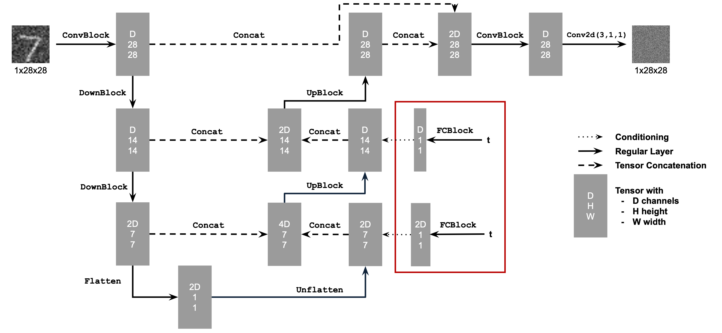
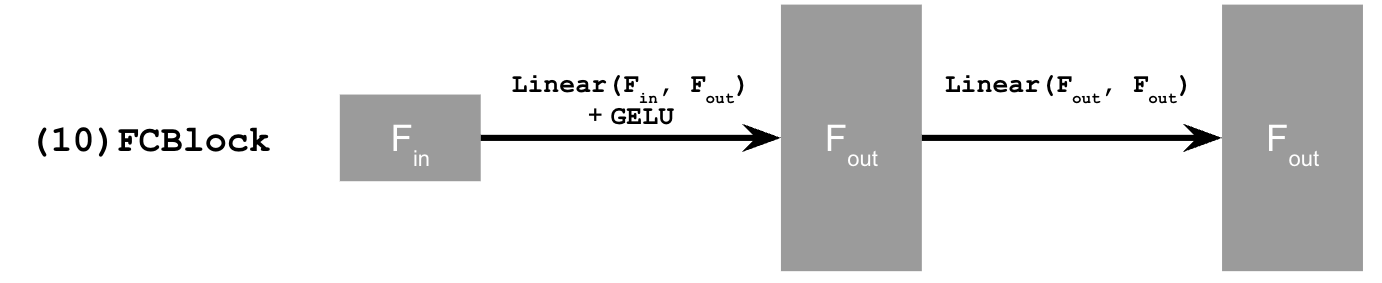
This uses a new operator called FCBlock (fully-connected
block) which we use to inject the conditioning signal into the UNet:
Train the Time Conditioned UNet
Training our time-conditioned UNet \(\epsilon_\theta(x_t, t)\) is now pretty easy. Basically, we pick a random image from the training set, a random \(t\), and train the denoiser to predict the noise in \(x_t\). We repeat this for different images and different t values until the model converges and we are happy.
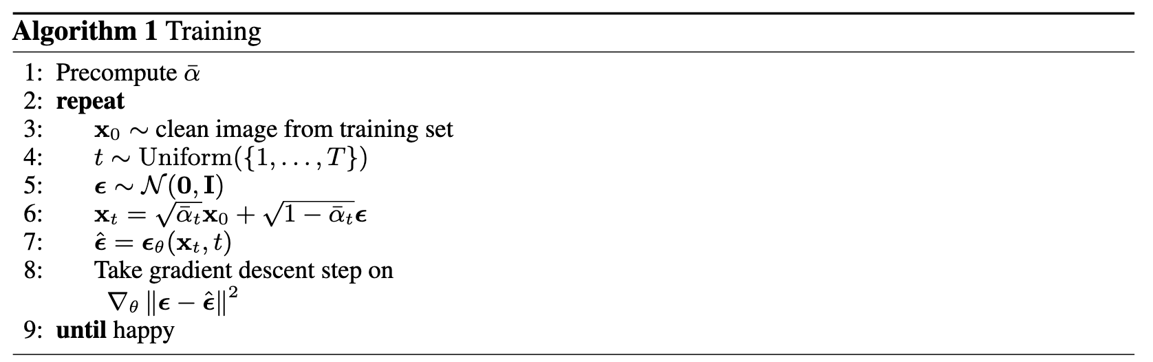
Objective: Train a time-conditioned UNet \(\epsilon_\theta(x_t, t)\) to predict the noise in \(x_t\) given a noisy image \(x_t\) and a timestep \(t\).
Dataset and dataloader: Use the MNIST dataset via
torchvision.datasets.MNISTwith flags to access training and test sets. Train only on the training set. Shuffle the dataset before creating the dataloader. Recommended batch size: 128. We'll train over our dataset for 20 epochs since this task is more difficult than part A.- As shown in algorithm B.1, you should only noise the image batches when fetched from the dataloader.
Model: Use the time-conditioned UNet architecture defined in section 2.1 with recommended hidden dimension \(D = 64\). Follow the diagram and pseudocode for how to inject the conditioning signal \(t\) into the UNet. Remember to normalize \(t\) before embedding it.
Optimizer: Use Adam optimizer with an initial learning rate of \(1 \times 10^{-3}\). We will be using an exponential learning rate scheduler with a gamma of \(0.1^{(1.0 / \text{num\_epochs})}\). This can be implemented using:
```python scheduler = torch.optim.lr_scheduler.ExponentialLR(...)
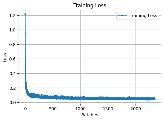
Here is the Time-Conditioned UNet training loss curve.
Sampling from the Time Conditioned UNet
The sampling process is very similar to part A, except we don't need to predict the variance like in the DeepFloyd model. Instead, we can use our list \(\beta\).
|
Sampled Image Train epoch=5 |
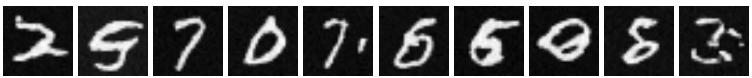
|
|
Sampled Image Train epoch=20 |
|
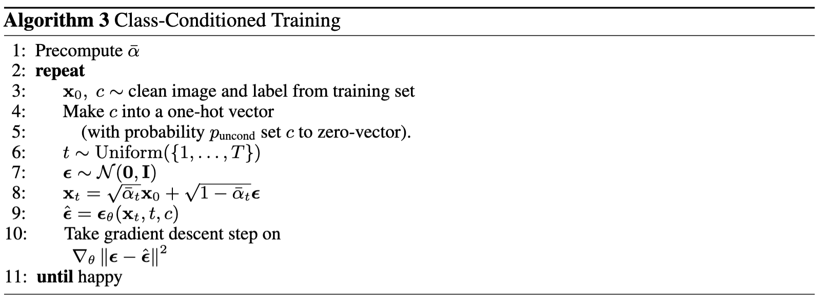
Adding Class-Conditioning to UNet
To make the results better and give us more control for image
generation, we can also optionally condition our UNet on the class of
the digit 0-9. This will require adding 2 more FCBlocks to
our UNet, but we suggest that for class-conditioning vector \(c\), you make it a one-hot vector instead
of a single scalar.
Because we still want our UNet to work without it being conditioned
on the class, we implement dropout where 10% of the time \((p_{\text{uncond}} = 0.1)\), we drop the
class conditioning vector \(c\) by
setting it to 0. Here is one way to condition our UNet \(\epsilon_\theta(x_t, t, c)\) on both time
\(t\) and class \(c\):
unflatten = c1 * unflatten + t1
Training for this section will be the same as time-only, with the only difference being the conditioning vector c and doing unconditional generation periodically.
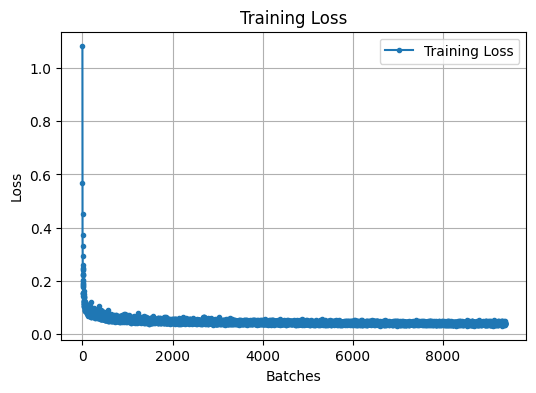
The training loss can be visualized as:
|
Sampled Image Train epoch=5 |
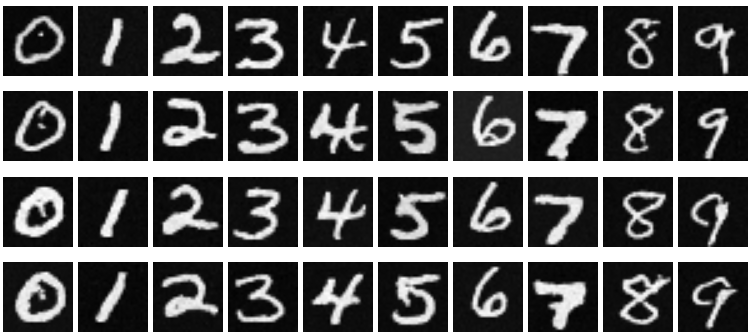
|
|
Sampled Image Train epoch=20 |
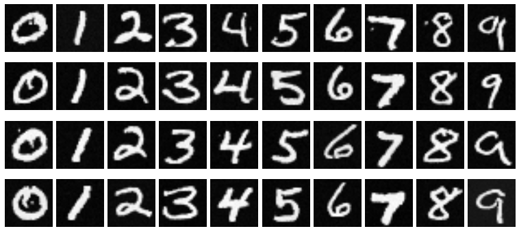
|
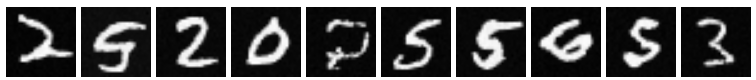
It seems great! It seems that this cutie little diffusion model has "learned" to write numbers!