CS188-Artificial Intelligence Midterm Review & Cheatsheet

 2024/10/16 

Midterm Review & Cheatsheet for CS 188 Fall 2024 | Introduction to Artificial Intelligence at UC Berkeley

Author: SimonXie2004.github.io

Resources

Download Cheatsheet (pdf)

Download Cheatsheet (pptx)

Lec1: Introduction

N/A

Lec2: Search

Reflex Agents V.S. Planning Agents:
1. Reflex Agents: Consider how the world IS
2. Planning Agents: Consider how the world WOULD BE
Properties of Agents
1. Completeness: Guaranteed to find a solution if one exists.
2. Optimality: Guaranteed to find the least cost path.
Definition of Search Problem: State Space, Successor Function, Start State & Goal Test
Definition of State Space: World State & Search State
State Space Graph: Nodes = states, Arcs = successors (action results)

Tree Search

Main Idea: Expand out potential nodes; Maintain a fringe of partial plans under consideration; Expand less nodes.
Key notions: Expansion, Expansion Strategy, Fringe

Common tree search patterns (Suppose b = branching factor, m = tree depth.) Nodes in search tree? \(\sum_{i=0}^{m}b^i = O(b^m)\) (For BFS, suppose s = depth of shallowest solution) (For Uniform Cost Search, suppose solution costs \(C^*\), min(arc_cost) = \(\epsilon\))

	Strategy	Fringe	Time	Memory	Completeness	Optimality
DFS	Expand deepest node first	LIFO Stack	\(O(b^m)\)	\(O(bm)\)	True (if no cycles)	False
BFS	Expand shallowest node first	FIFO Queue	\(O(b^s)\)	\(O(b^s)\)	True	True (if cost=1)
UCS	Expand cheapest node first	Priority Queue (p=cumulative cost)	\(O(C^*/\epsilon)\)	\(O(b^{C^*/\epsilon})\)	True	True

Special Idea: Iterative Deepening Run DFS(depth_limit=1), DFS(depth_limit=2), ...
Example Problem: Pancake flipping; Cost: Number of pancakes flipped

Graph Search
1. Idea: never expand a state twice
2. Method: record set of expanded states where elements = (state, cost). If a node popped from queue is NOT visited, visit it. If a node popped from queue is visited, check its cost. If the cost if lower, expand it. Else skip it.

Lec3: Informed Search

Definition of heuristic: function that estimates how close a state is to a goal; Problem specific!
Example heuristics: (Relaxed-problem heuristic)
1. Pancake flipping: heuristic = the number of largest pancake that is still out of place
2. Dot-Eating Pacman: heuristic = the sum of all weights in a MST (of dots & current coordinate)
3. Classic 8 Puzzle: heuristic = number of tiles misplaced
4. Easy 8 Puzzle (allow tile to be piled intermediately): heuristic = total Manhattan distance
Remark: Can't use actual cost as heuristic, since you have to solve that first!
Comparison of algorithms:
1. Greedy Search: expand closest node (to goal); orders by forward cost h(n); suboptimal
2. UCS: expand closest node (to start state); orders by backward cost g(n); suboptimal
3. A* Search: orders by sum f(n) = g(n) + h(n)
A* Search
1. When to stop: Only if we dequeue a goal
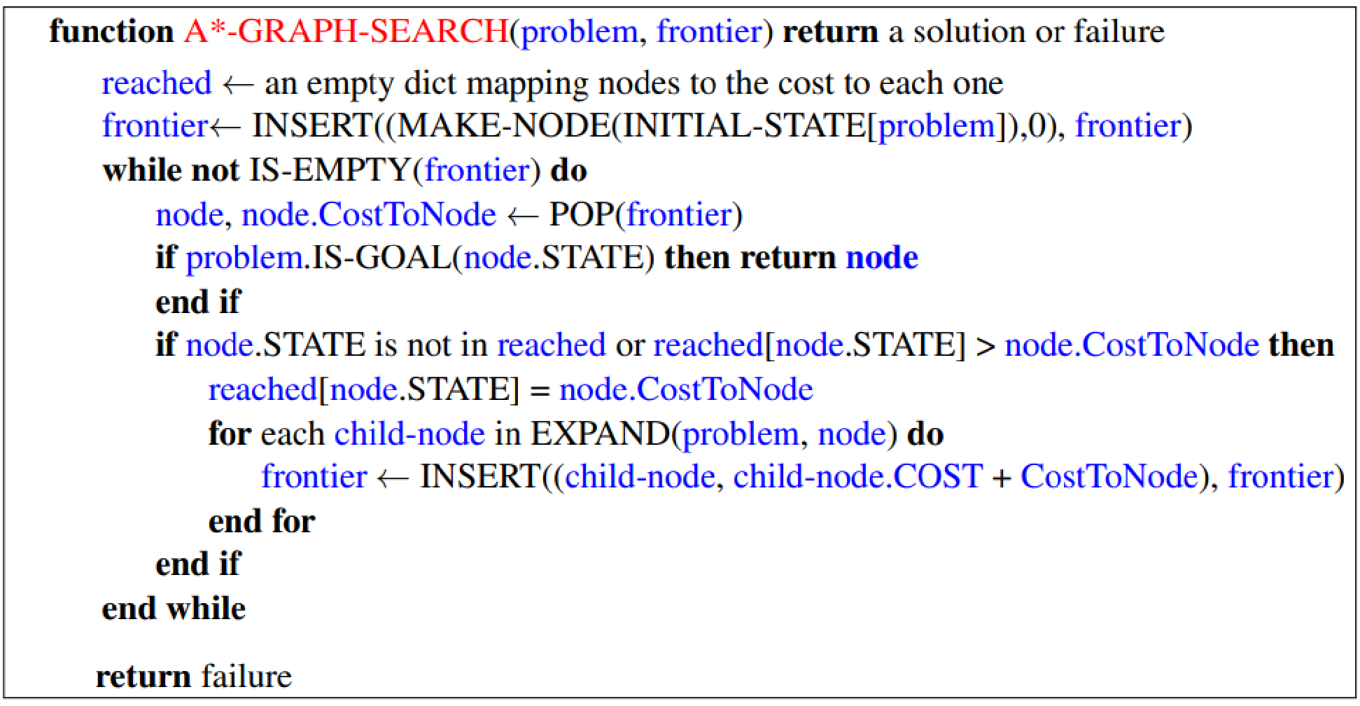
2. Admissible (optimistic) heuristic: \(\forall n, 0 \le h(n) \le h^*(n)\). A* Tree Search is optimal if heuristic is admissible. Proof: Step 1, Step 2.
3. Consistent heuristic: \(\forall A, B, h(A) - h(B) \le cost(A, B)\) A* Graph Search is optimal if heuristic is consistent. Proof: Sketch, Step 1, Step 2
Semi-Lattice of Heuristics
1. Dominance: define \(h_a \ge h_c\) if \(\forall n, h_a(n) \ge h_c(n)\)
2. Heuristics form semi-lattice because: \(\forall h(n) = max(h_a(n), h_b(n)) \in H\)
3. Bottom of lattice is zero-heuristic. Top of lattice is exact-heuristic

Lec 4-5: Constraint Satisfaction Problems

Definition of CSP Problems: (A special subset of search problems)
1. State: Varibles {Xi}, with values from domain D
2. Goal Test: set of constraints specifying allowable combinations of values
Example of CSP Problems:
1. N-Queens
  
  Formulation 1: Variables: Xij, Domains: {0, 1}, Constraints: \(\forall i, j, k, (X_{ij}, X_{jk}) \neq (1, 1), \cdots\) and \(\sum_{i, j}X_{ij} = N\)
  
  Formulation 2: Variables Qk, Domains: {1, ..., N}, Constraints: \(\forall (i, j), \text{non-threatening}(Q_i, Q_j)\)
2. Cryptarithmetic
Constraint Graph:
1. Circle nodes = Variables; Rectangular nodes = Constraints.
2. If there is a relation between some variables, they are connected to a constraint node.
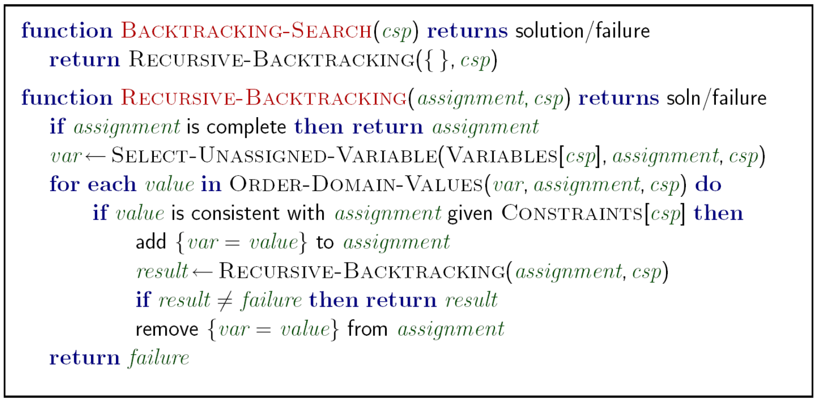
Simple Backtracking Search
1. One variable at a time
2. Check constraints as you go. (Only consider constraints not conflicting to previous assignments)
Simple Backtracking Algorithm

= DFS + variable-ordering + fail-on-violation
Filtering & Arc Consistency
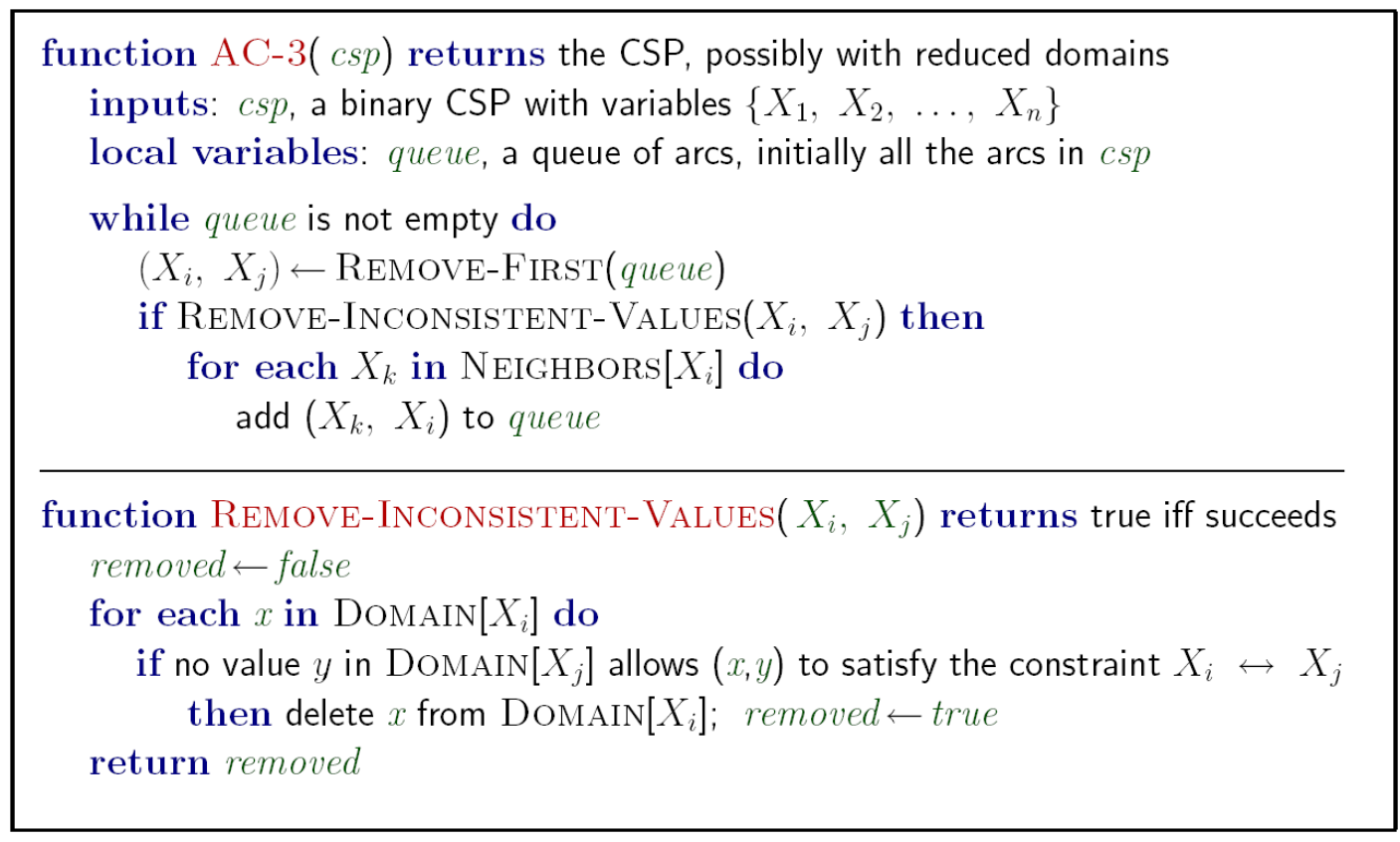
1. Definition: Arc \(X \rightarrow Y\) is consistent if \(\forall x \in X, \exists y \in Y\) that could be assigned. (Basically X is enforcing constraints on Y)
2. Filtering: Forward Checking: Enforcing consistency of arcs pointing to each new assignment
3. Filtering: Constraint Propagation: If X loses a Value, neighbors of X need to be rechecked.
4. Usage: run arc consistency as a preprocessor or after each assignment
5. Algorithm with Runtime \(O(n^2d^3)\):
Advanced Definition: K-Consistency
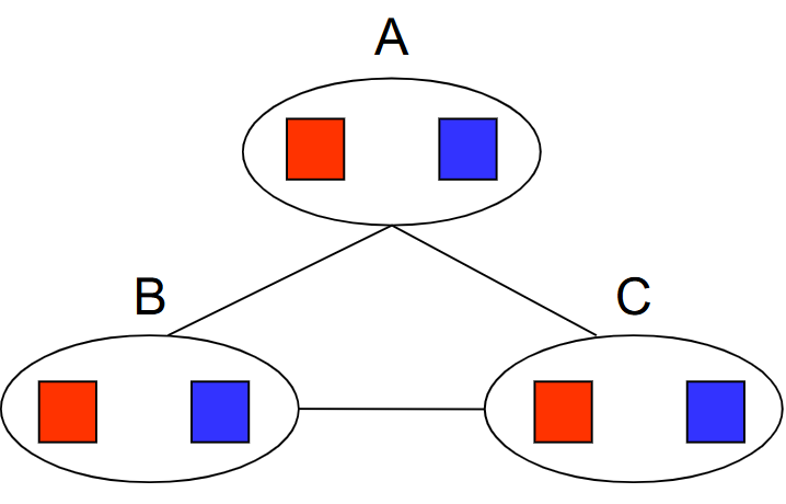
1. K-Consistency: For each k nodes, any consistent assignment to k-1 nodes can be extended to kth node.
2. Example of being NOT 3-consistent:
3. Strong K-Consistency: also k-1, k-2, ..., 1-Consistent; Can be solved immediately without searching
4. Problems of Arc-consistency: only considers 2-consitency
Advanced Arc-Consistency: Ordering
1. Variable Ordering: MRV (Minimum Remaining Value): Choose the variable with fewest legal left values in domain
2. Value Ordering: LCV (Least Constraining Value): Choose the value that rules out fewest values in remaining variables.
  
  (May require re-running filtering.)
Advanced Arc-Consistency: Observing Problem Structure
1. Suppose graph of n variables can be broken into subproblems with c variables: Can solve in \(O(\frac{n}{c}) \cdot O(d^c)\)
2. Suppose graph is a tree: Can solve in \(O(nd^2)\). Method as follows
  1. Remove backward: For i = n : 2, apply RemoveInconsistent(Parent(Xi),Xi)
  2. Assign forward: For i = 1 : n, assign Xi consistently with Parent(Xi)
  3. *Remark: After backward pass, all root-to-leaf are consistent. Forward assignment will not backtrack.
Advanced Arc-Consistency: Improving Problem Structure
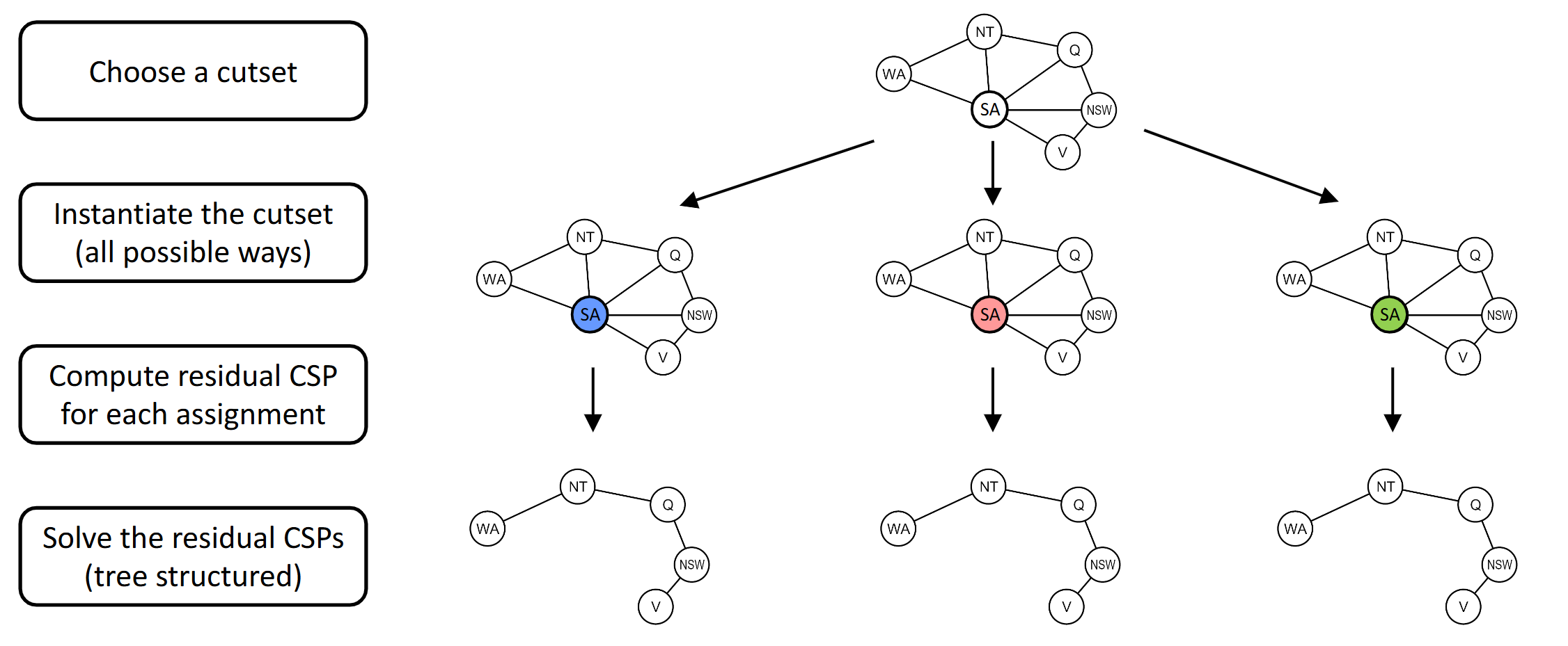
1. Idea: Initiate a variable and prune its neighbors' domains.
2. Method: instantiate a set of vars such that remaining constraint graph is a tree (cutset conditioning)
3. Runtime: \(O(d^c \cdot (n-c)d^2)\) to solve CSP.
Iterative Methods: No Fringe!
1. Local Search
  
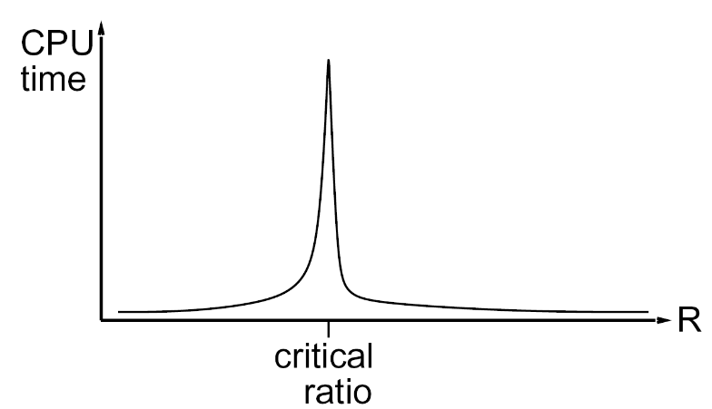
  Algorithm: While not solved, randomly select any conflicted variable. Assign value by min-conflicts heuristic.
  
  Performance: can solve n-queens in almost constant time for arbitrary n with high probability, except a few of them.
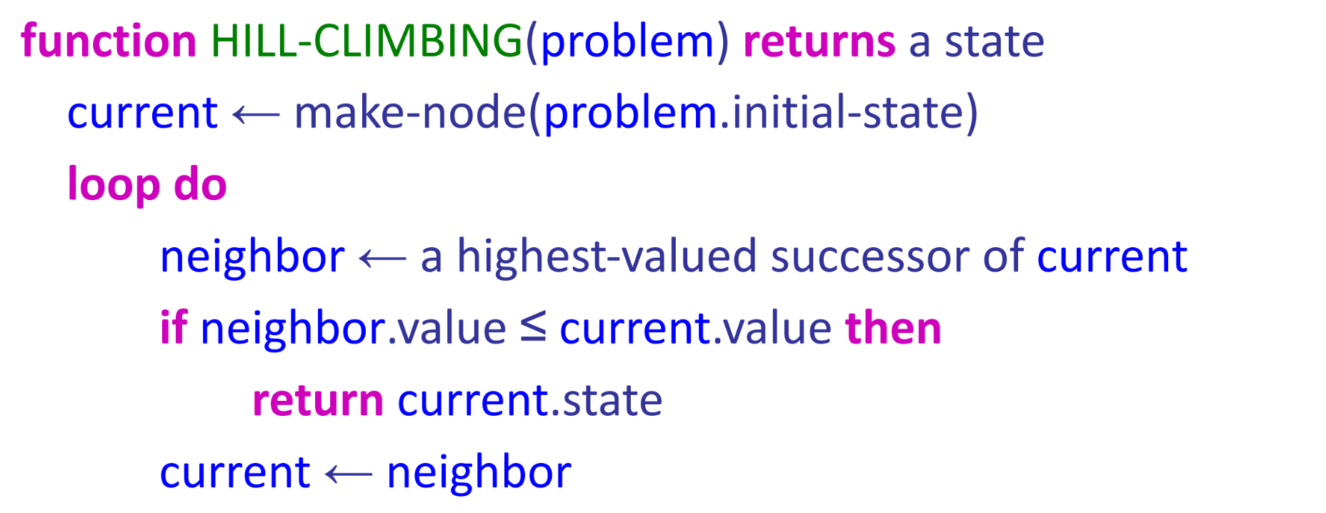
2. Hill-climbing
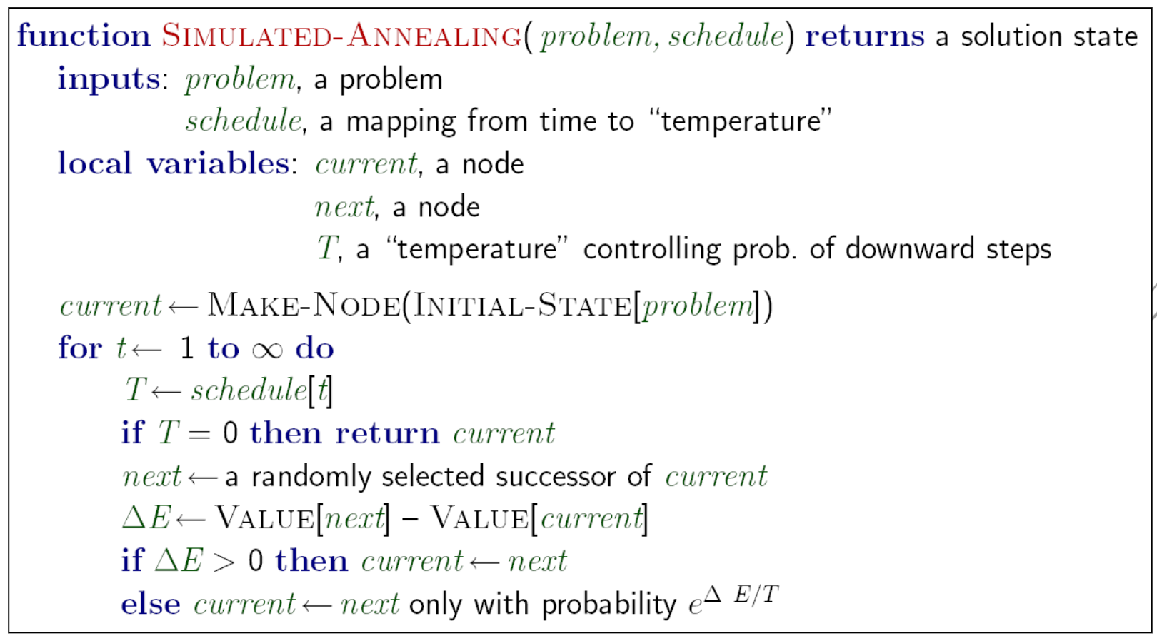
3. Simulated Annealing
  
  Remark: Stationary distribution: \(p(x) \propto e^{\frac{E(x)}{kT}}\)
4. Genetic Algorithms

Lec 6: Simple Game Trees (Minimax)

Zero-Sum Games V.S. General Games: Opposite utilities v.s. Independent utilities
1. Examples of Zero-Sum Games: Tic-tac-toe, chess, checkers, ...
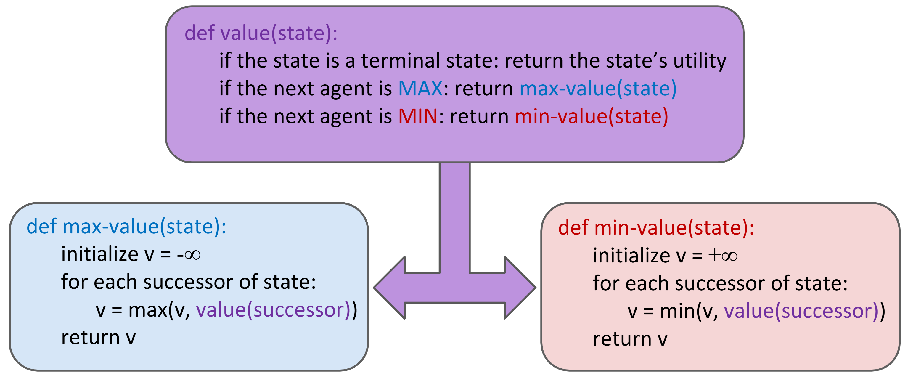
Value of State: Best achievable outcome (utility) from that state.
1. For MAX players, \(max_{s' \in \text{children}(s)} V(s')\); For MIN players, min...
Search Strategy: Minimax
Minimax properties:
1. Optimal against perfect player. Sub-optimal otherwise.
2. Time: \(O(b^m)\), Space: \(O(bm)\)
Alpha-Beta Pruning
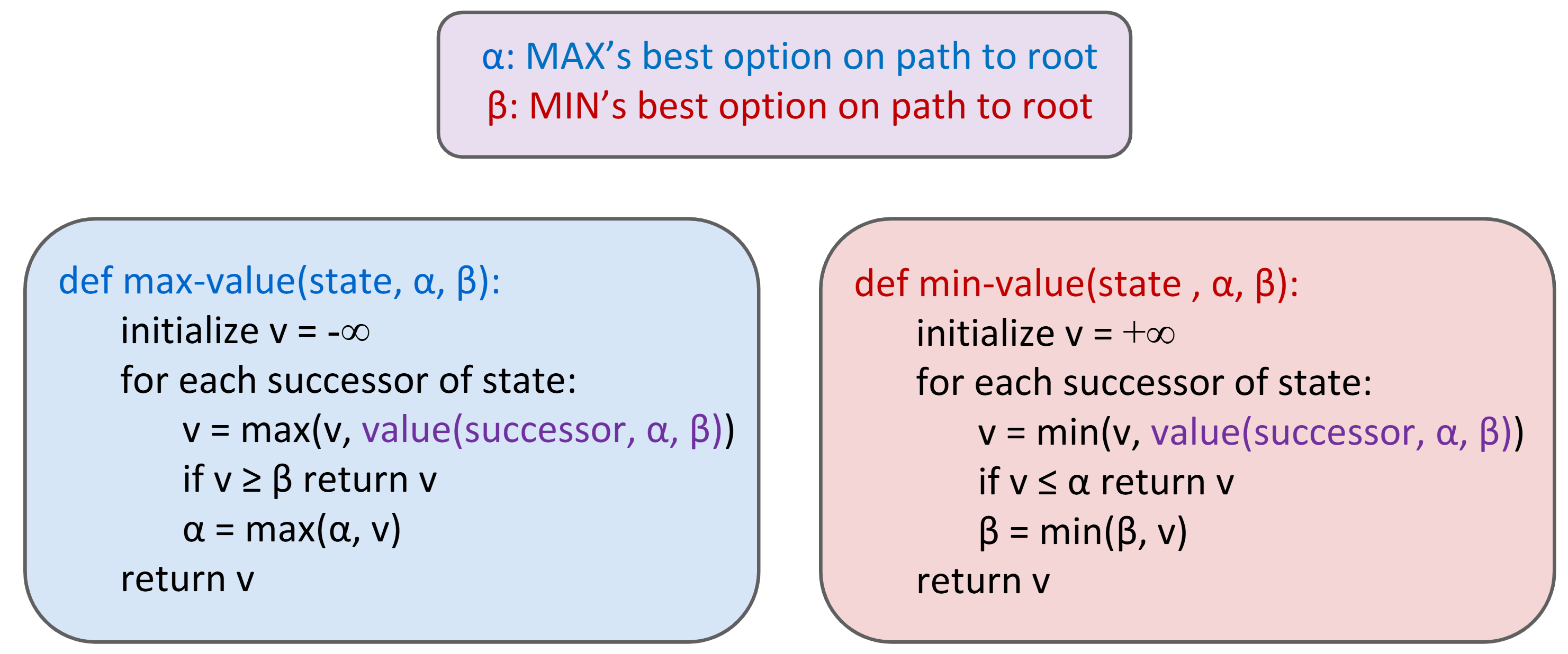
1. Algorithm:
2. Properties:
  1. Meaning of Alpha: maximum reward for MAX players, best option so far for MAX player
  2. Meaning of Beta: minimum loss for MIN players, best option so far for MIN player
  3. Have no effect on root value; intermediate values might be wrong.
  4. With perfect ordering, time complexity drops to \(O(b^{m/2})\)
Depth-Limited Minimax: replace terminal utilities with an evaluation function for non-terminate positions
1. Evaluation Functions: weighted sum of features observed
Iterative Deepening: run minimax with depth_limit = 1, 2, 3, ... until timeout

Lec 7: More Game Trees (Expectimax, Utilities, Multiplayer)

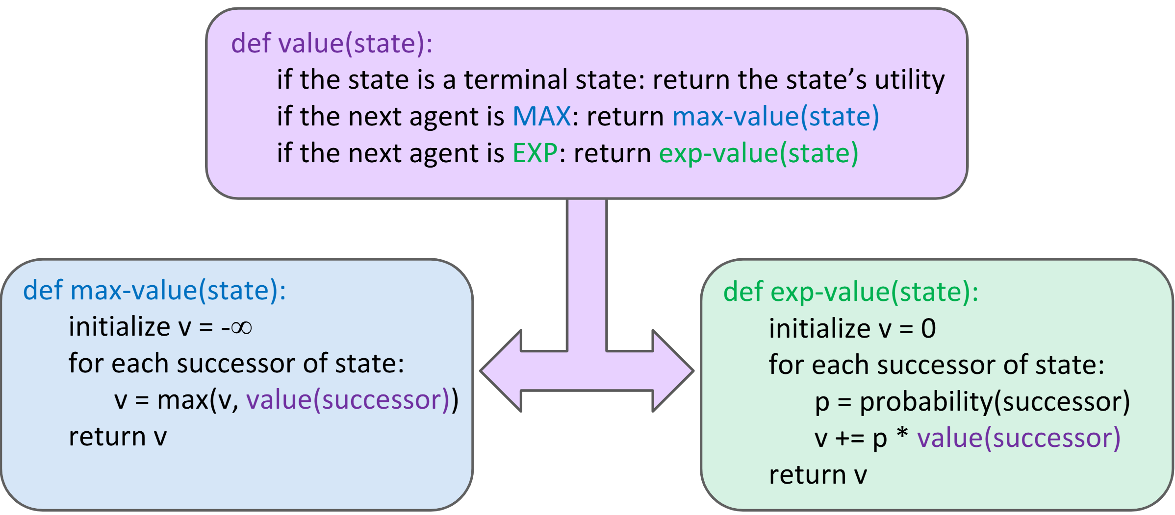
Expetimax Algorithm:
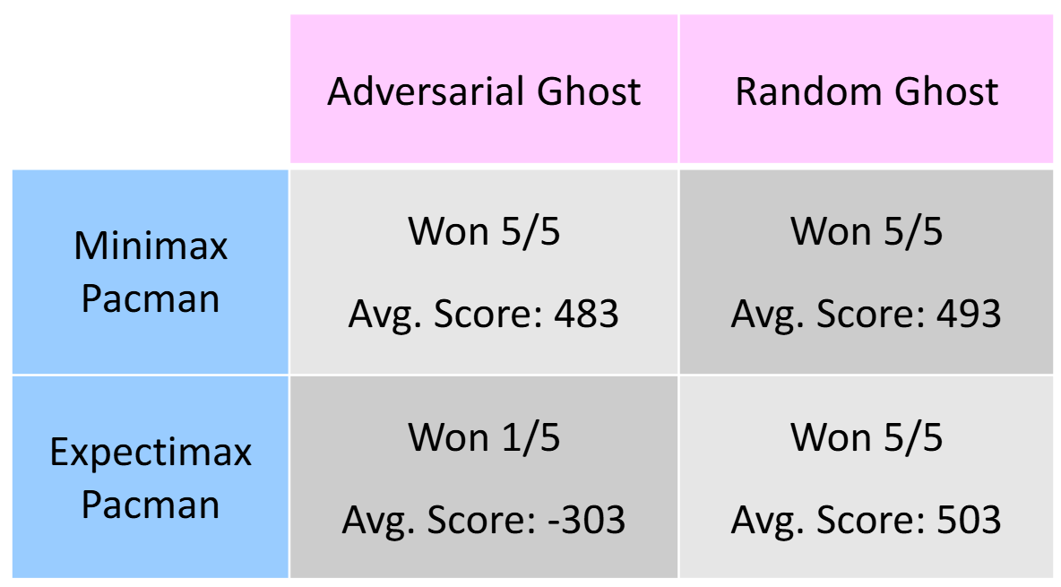
Assumptions V.S. Reality: Rational & Irrational Agents
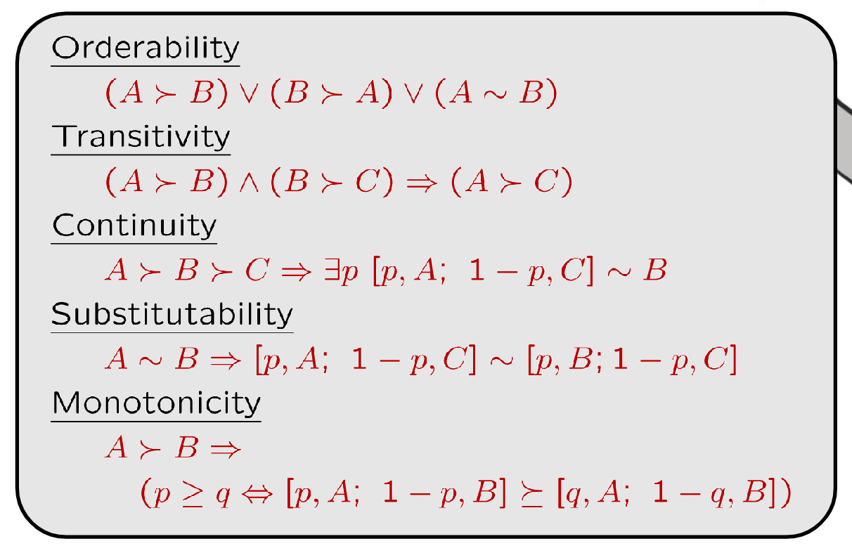
Axioms of Rationality
MEU Principle

Given any preferences satisfying these constraints, there exists a real-valued function U such that:
Risk-adverse v.s. Risk-prone
1. Def. \(L = [p, X, 1-p, Y]\)
2. If \(U(L) < U(EMV(L))\), risk-adverse
  
  Where \(U(L) = pU(X) + (1-p)U(Y)\), \(U(EMV(L)) = U(pX + (1-p)Y)\)
  
  i.e. if U is concave, like y=log2x, then risk-adverse
3. Otherwise, risk-prone.
  
  i.e. if U is convex, like y=x^2, then risk-prone

Lec 8-9: Markov Decision Processes

MDP World: Noisy movement, maze-like problem, receives rewards.
1. "Markov": Successor only depends on current state (not the history)
MDP World Definition:
1. States, Actions
2. Transition Function \(T(s, a, s')\) or \(Pr(s' | s, a)\), Reward Function \(R(s, a, s')\)
3. Start State, (Probably) Terminal State
MDP Target: optimal policy \(\pi^*: S \rightarrow A\)
Discounting: Earlier is Better! No infinity rewards!
1. \(U([r_0, \cdots, r_\inf]) = \sum_{t=0}^\inf \gamma^tr_t =\le R_{\text{max}} / (1-\gamma)\)
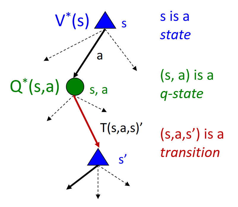
MDP Search Trees:
1. Value of State: expected utility starting in s and acting optimally.
  
  \(V^*(s) = \max_a Q^*(s, a)\)
2. Value of Q-State: expected utility starting out having taken action a from state s and (thereafter) acting optimally.
  
  \(Q^*(s, a) = \sum_{s'}T(s, a, s')[R(s, a, s' + \gamma V^*(s'))]\)
3. Optimal Policy: \(\pi^*(s)\)
Solving MDP Equations: Value Iteration
1. Bellman Equation: \(V^*(s) = \max_a \sum_{s'}T(s, a, s')[R(s, a, s') + \gamma V(s')]\)
2. Value Calculation: \(V_{k+1}(s) \leftarrow \max_a \sum_{s'}T(s, a, s')[R(s, a, s') + \gamma V_k(s')]\)
3. Policy Extraction: \(\pi^*(s) = \arg \max_{a} \sum_{s'} T(s, a, s')[R(s, a, s') + \gamma V^*(s')]\)
4. Complexity (of each iteration): \(O(S^2A)\)
5. Must converge to optimal values. Policy may converge much earlier.
Solving MDP Equations: Q-Value Iteration
1. Bellman Equation: \(Q^*(s, a) = \sum_{s'} T(s, a, s') [R(s, a, s' + \gamma \max_{a'} Q^*(s', a'))]\)
2. Policy Extraction: \(\pi^*(s) = \arg \max_{a} Q^*(s, a)\)
MDP Policy Evalutaion: Evaluating V for fixed policy \(\pi\)
1. Idea 1: remove the max'es from Bellman, iterating \(V_{k+1}(s) \leftarrow \sum_{s'}T(s, \pi(s), s')[R(s, \pi(s), s') + \gamma V_k(s')]\)
2. Idea 2: is a linear system. Use a linear system solver.
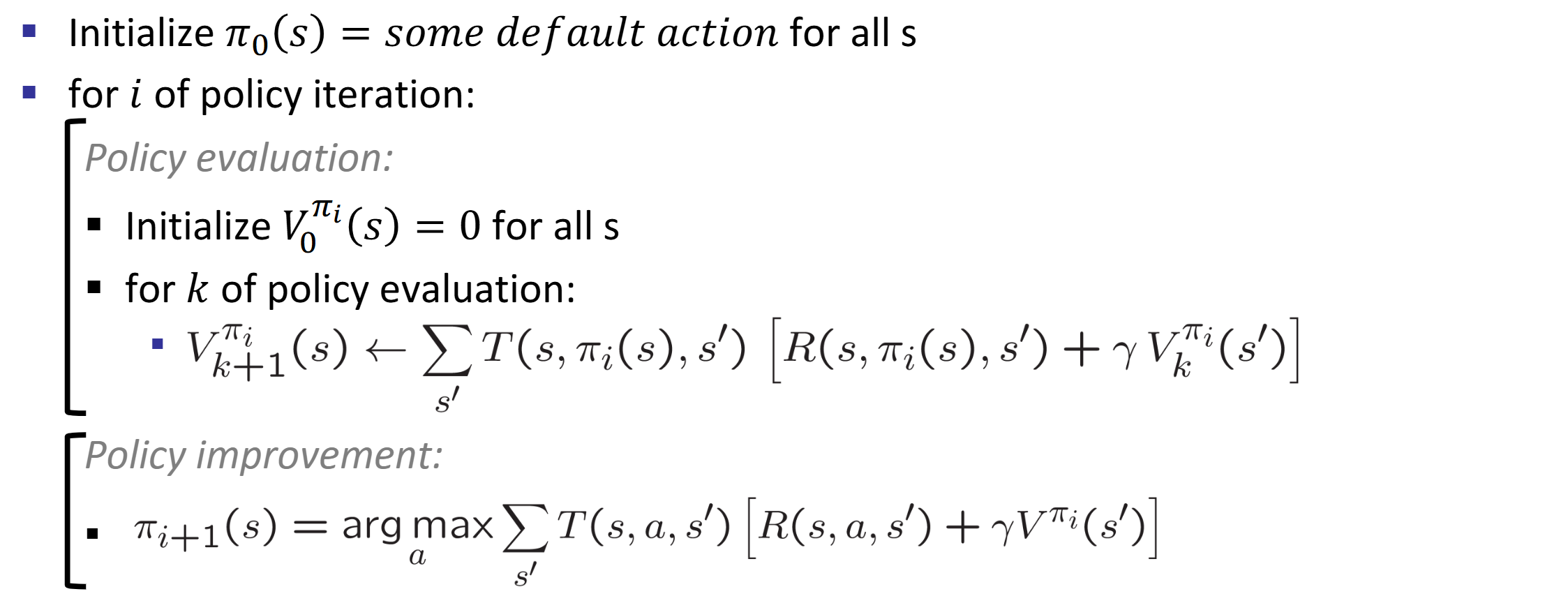
Solving MDP Equations: Policy Iteration
1. Idea: Update Policy & Value meanwhile, much much faster!
2. Algorithm:

Lec 10-11: Reinforcement Learning

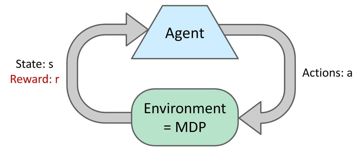
Intuition: Suppose we know nothing about the world. Don't know T or R.
Passive RL I: Model-Based RL
1. Count outcomes s' for each s, a; Record R;
2. Calculate MDP through any iteration
3. Run policy. If not satisfied, add data and goto step 1
Passive RL II: Model-Free RL (Direct Evaluation, Sample-Based Bellman Updates)
1. Intuition: Direct evaluation from samples. improve our estimate of V by computing averages of samples.
2. Input: fixed policy \(\pi(s)\)
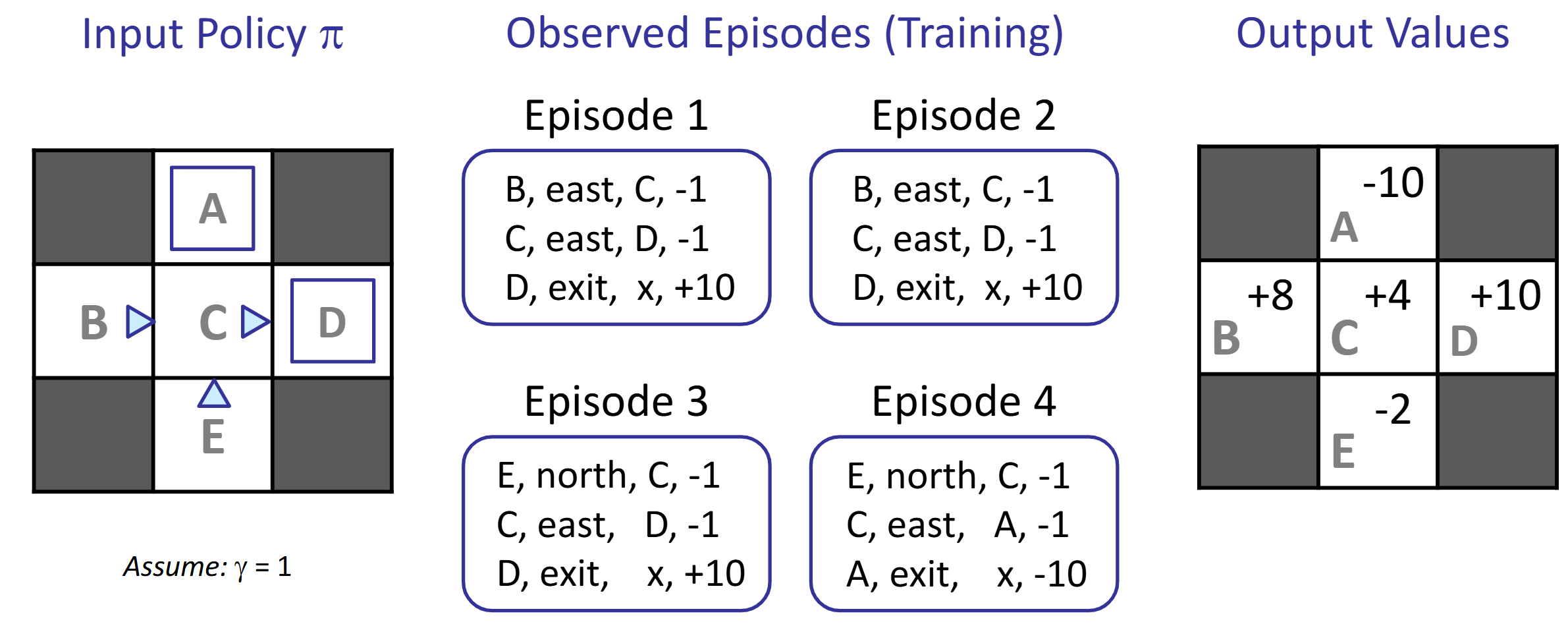
3. Act according to \(\pi\). Each time we visit a state, write down what the sum of discounted rewards turned out to be.
4. Average the samples, we get estimate of \(V(s)\)
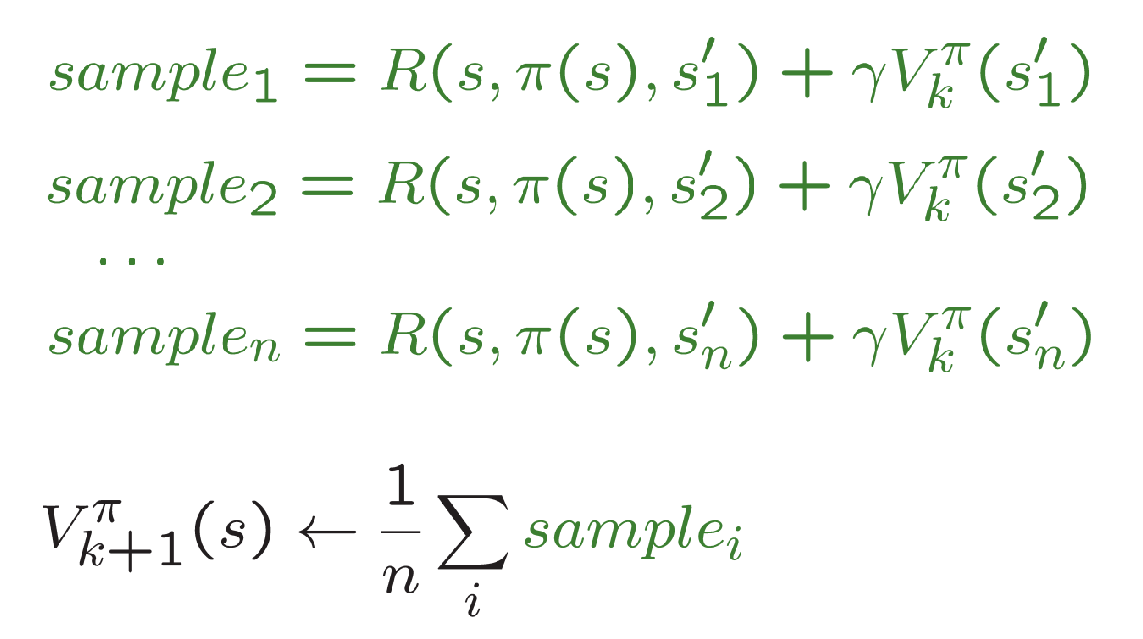
5. Problem: wastes information about state connections. Each state learned separately. Takes long time.
Passive RL II: Model-Free RL (Temporal Difference Learning)
1. Intuition: learn from everywhere / every experience.
  
  Recent samples are more important. \(\hat{x}_n = (1-a) x_{n-1} + ax_n\)
2. Update:
3. Decreasing learning rate (alpha) converges
4. Problem: Can't do policy extraction, can't calculate \(Q(s, a)\) without T or R
5. Idea: learn Q-values directly! Make action selection model-free too!
Passive RL III: Model-Free RL (Q-Learning + Time Difference Learning)
1. Intuition: Learn as you go.
2. Update:
  1. Receive a sample (s, a, s', r)
  2. Let sample = \(R(s, a, s') + \gamma \max_{a'} Q(s', a')\)
  3. Incorporate new estimate into a running average: \(Q(s, a) \leftarrow (1 - a) Q(s,a) + a \cdot \text{sample}\)
  4. Another representation: \(Q(s, a) \leftarrow Q(s, a) + a \cdot \text{Difference}\) where diff = sample - orig
3. This is off-policy learning!
Active RL: How to act to collect data
1. Exploration schemes: eps-greedy
  1. With probability \(\epsilon\), act randomly from all options
  2. With probability \(1 - \epsilon\), act on current policy
2. Exploration functions: use an optimistic utility instead of real utility
  1. Def. optimistic utility \(f(u, n) = u + k / n\), suppose u = value estimate, n = visit count
  2. Modified Q-Update: \(Q(s, a) \leftarrow_a R(s, a, s') + \gamma \max_{a'} f(Q(s', a'), N(s', a'))\)
3. Measuring total mistake cost: sum of difference between expected rewards and suboptimality rewards.
Scaling up RL: Approximate Q Learning
1. State space too large & sparse? Use linear functions to approximately learn \(Q(s,a)\) or \(V(s)\)
2. Definition: \(Q(s, a) = w_1f_1(s, a) + w_2f_2(s, a) + ...\)
3. Q-learning with linear Q-fuctions:
  
  Transition := (s, a, r, s')
  
  Difference := \([r + \gamma \max_{a'}Q(s', a')] - Q(s, a)\)
  
  Approx. Update weight: \(w_i \leftarrow w_i + a \cdot \text{Difference} \cdot f_i(s, a)\)