
Overview
This is an implementation of a physically-based cloth simulator, with core features of:
- Mass-and-Spring Based Cloth Definition
- Simulation via Numerical Integration
- Collision with Objects
- Self-Collision through Spatial Hashmap
- Shaders (Phong, Bump, Displacement, Environment, ...)
Part 1: Masses and Springs
Definition
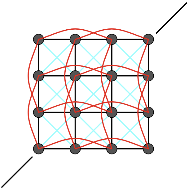
We define a cloth as a Mass-and-Spring system, with the following constraints:
Structural Spring: Between any adjacent point masses.
Shearing Spring: Between any diagonally adjacent point masses.
Bending Spring: Between any point masses that are two steps apart.
Result Gallery
|
|

|
|
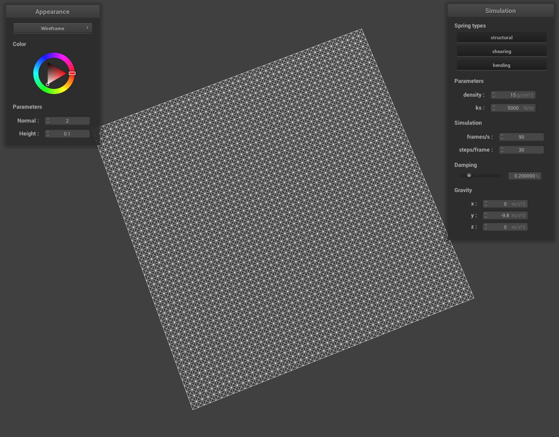
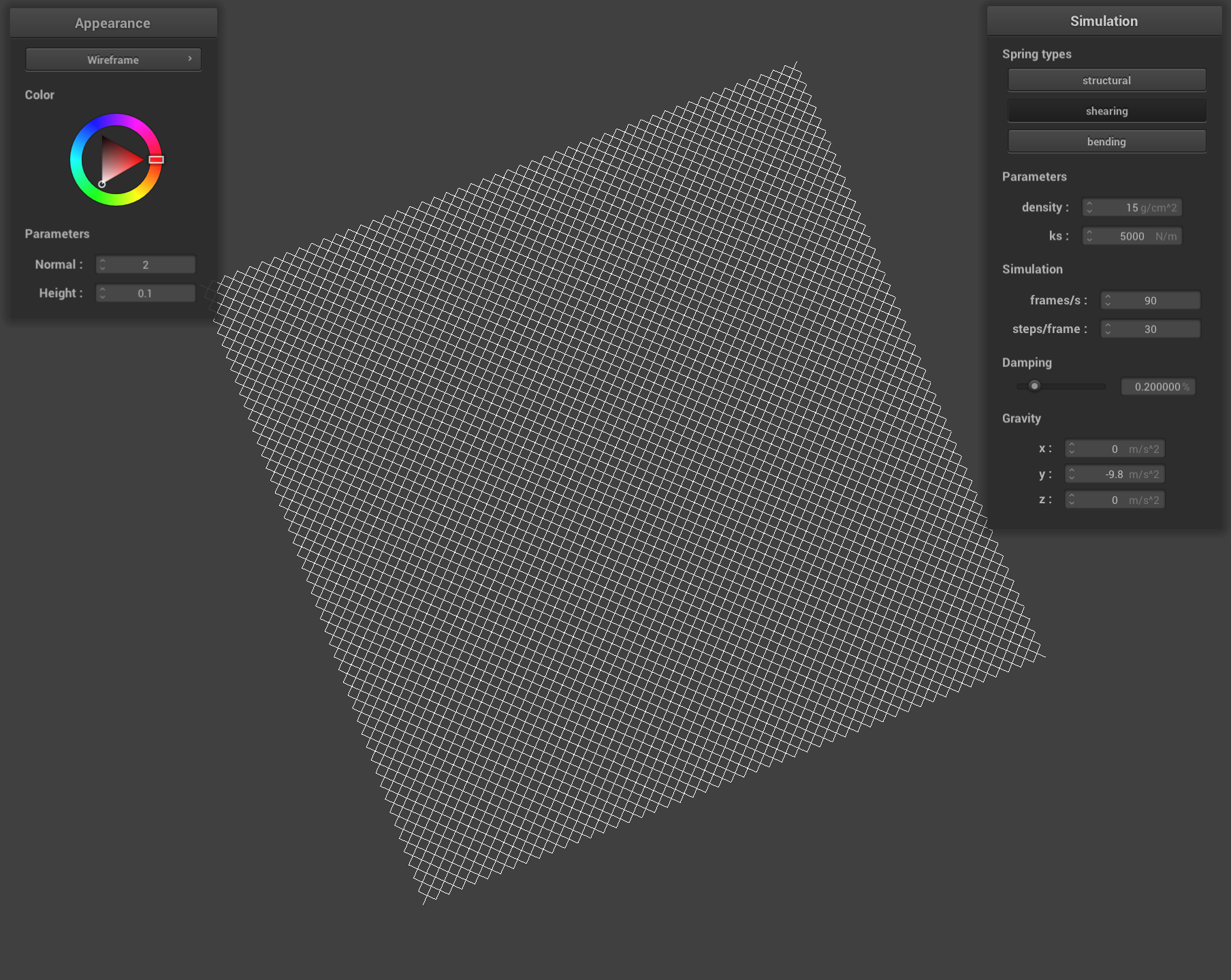
| All constraints |
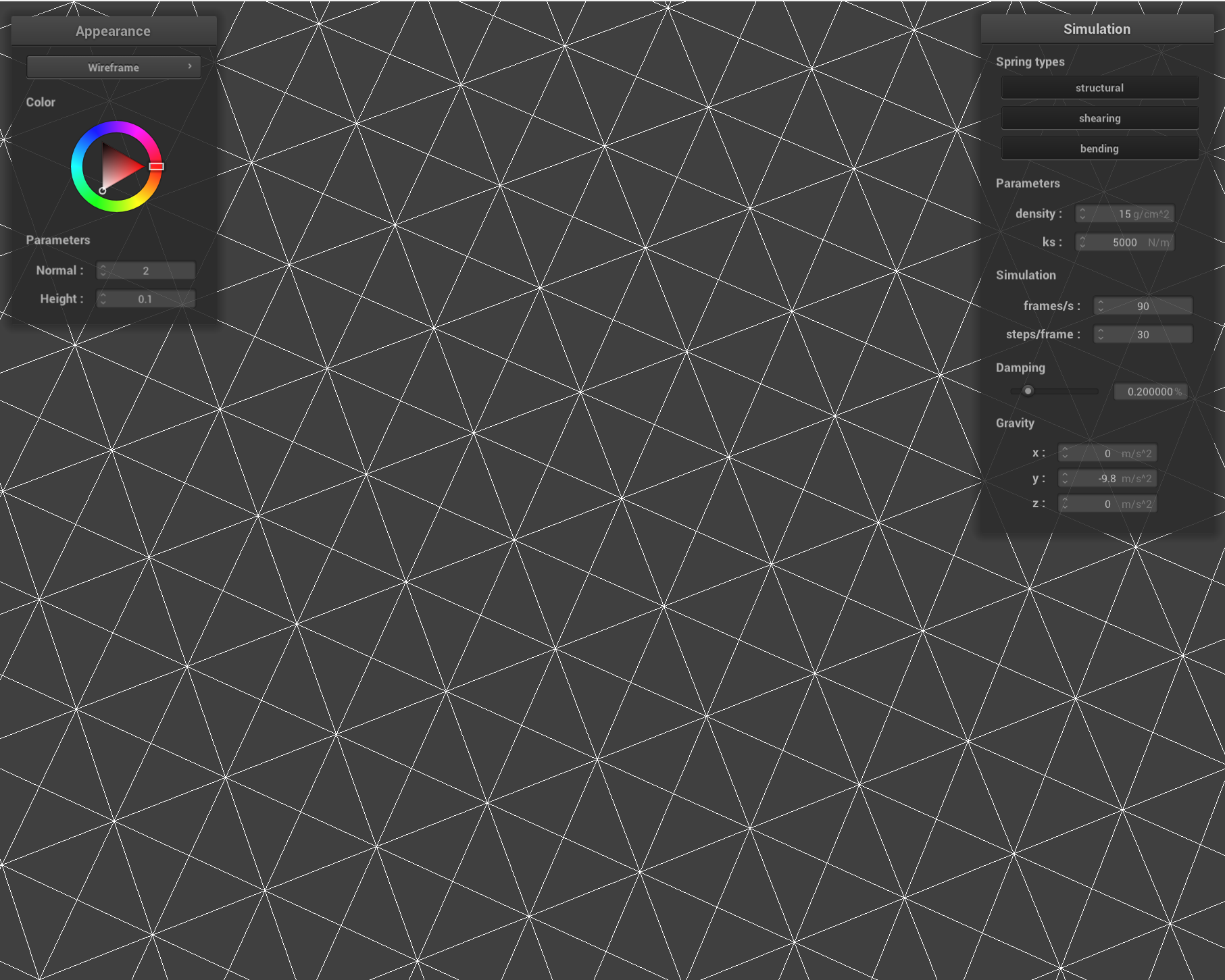
Closer lookup of all constraints |
Bending and Structural constraints | Shearing constraints |
Screenshots of scene/pinned2.json, showing the constraints.
Part 2: Verlet Integration
Algorithm
The Verlet integration combines from two parts:
First, update all point masses' forces. Algorithm:
- For all
springinsprings:- Calculate force by Hooke's law.
- Apply the force to the connected point masses:
pm_a->force += fpm_b->force -= f
Then, integrate the new position for each point mass using Verlet integration. Algorithm:
- For all
point_massinpoint_masses:- Compute acceleration:
a = total_force / mass - Store the current position:
Vector3 temp = position - Update position using damped Verlet integration:
position += (1 - damping) * (position - last_position) + a * delta_t^2 - Update last position:
last_position = temp
- Compute acceleration:
This approach approximates velocity as the difference between the
current and previous positions. The damping term helps
simulate energy loss due to internal friction, air resistance, or
material properties.
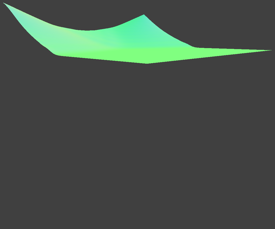
Result Gallery
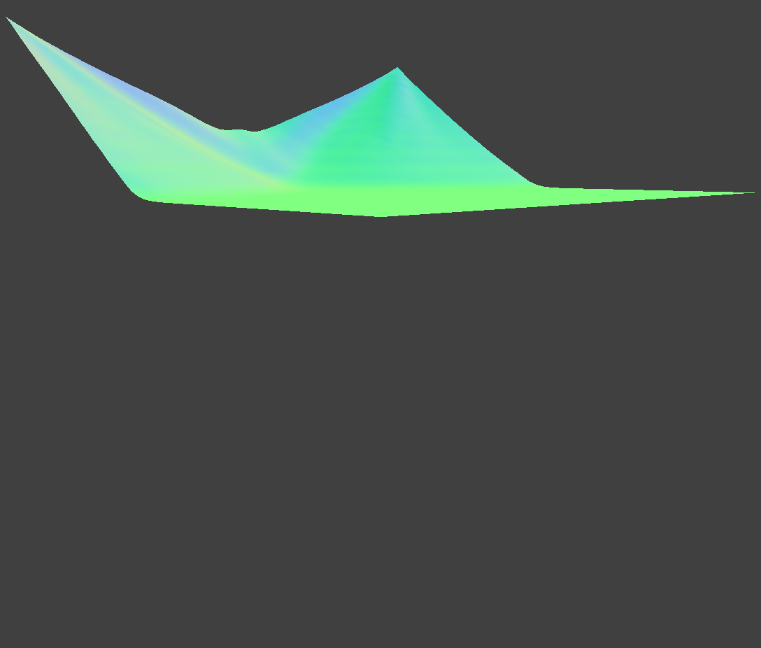
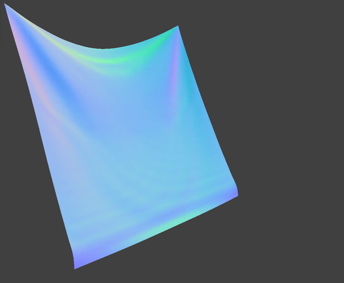
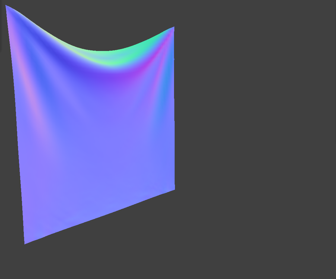
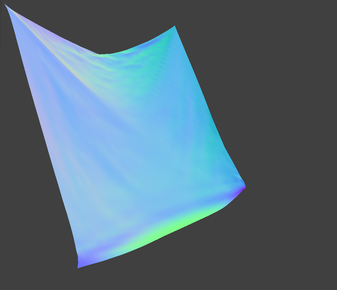
| Default: Ks = 5000 N/m, density = 15 g/cm^2, Damping = 0.2 | ||
|
|
|
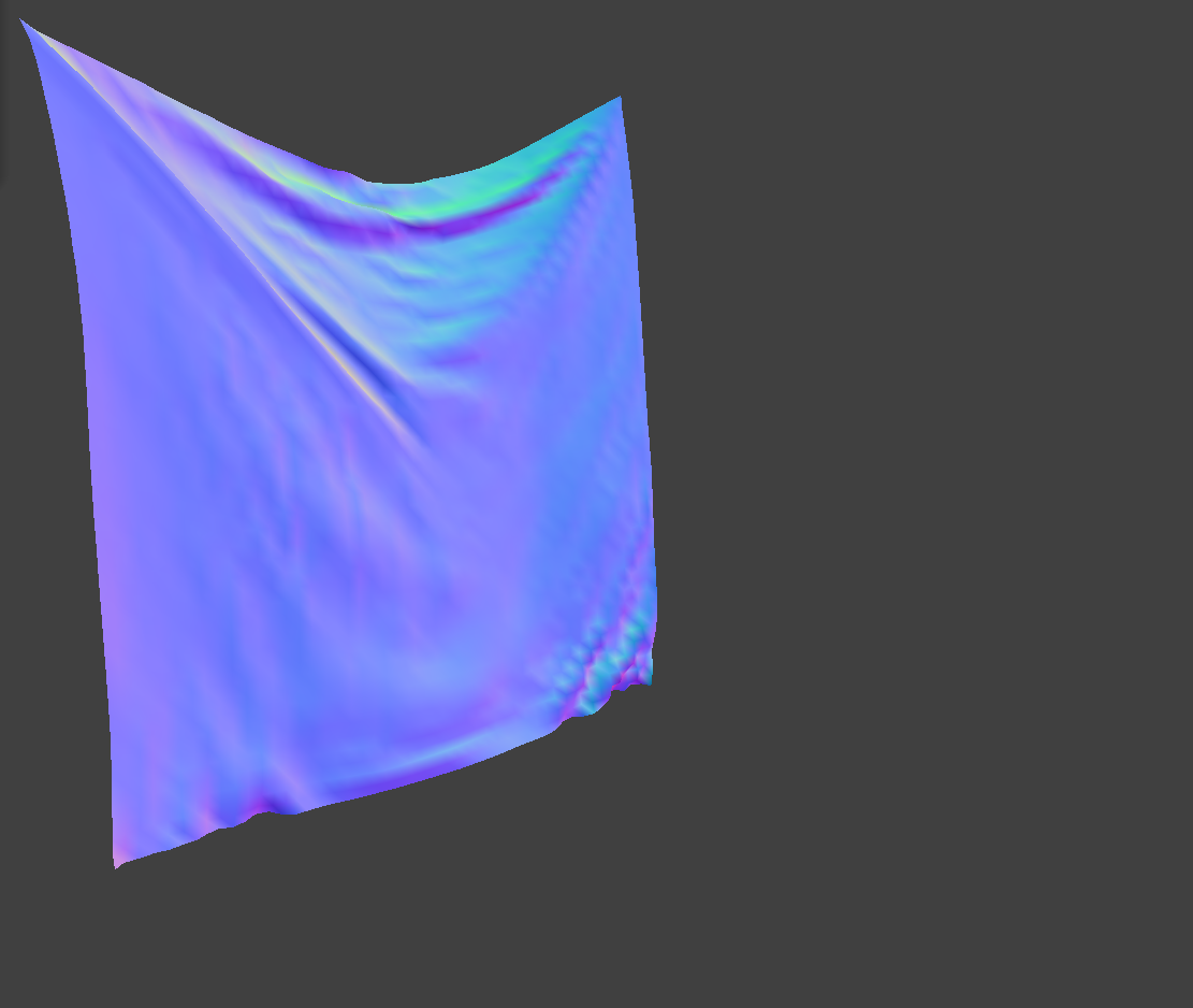
| Higher Ks = 50000 N/m | ||
|
|
|
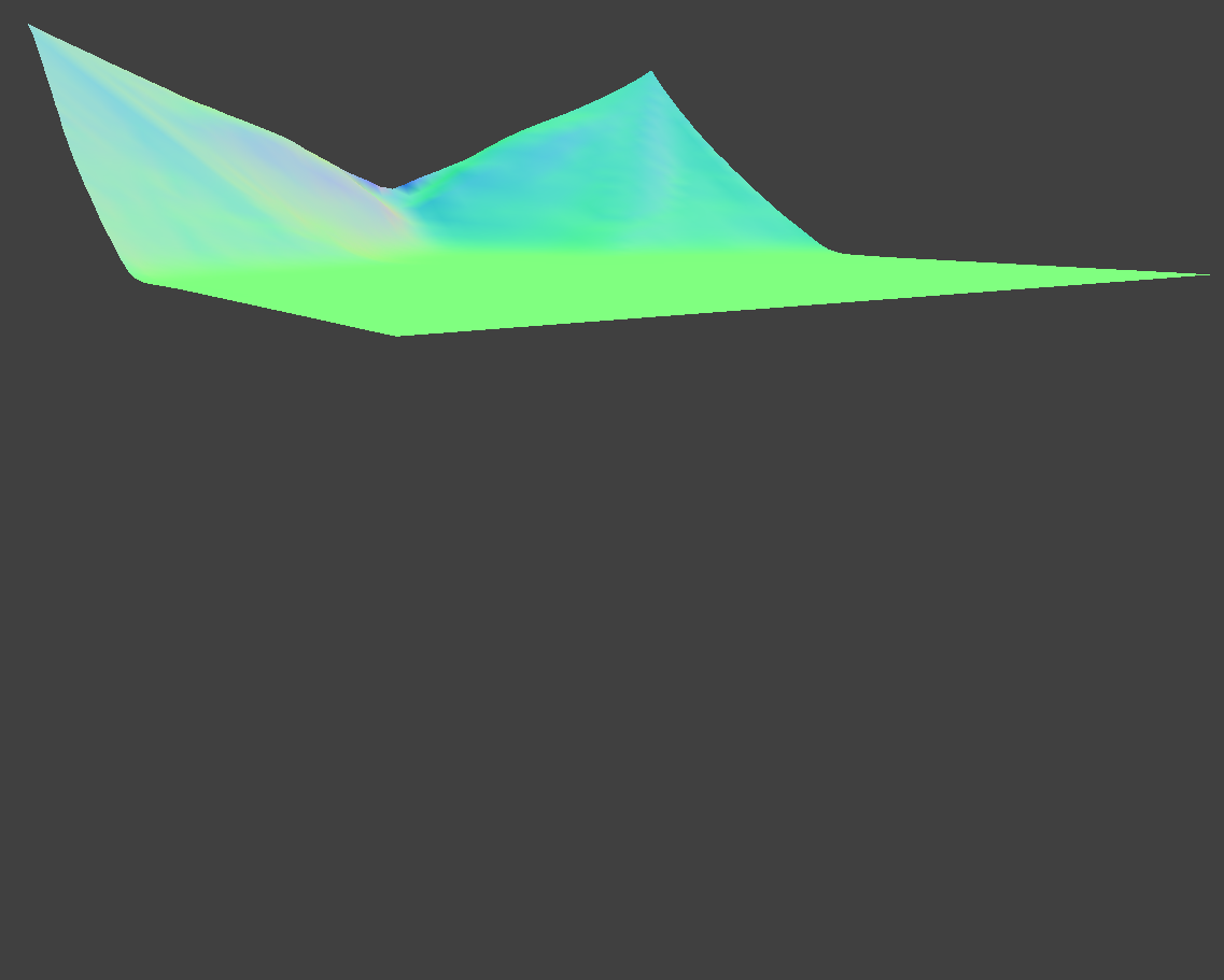
| Lower Ks = 500 N/m | ||
|
|
|
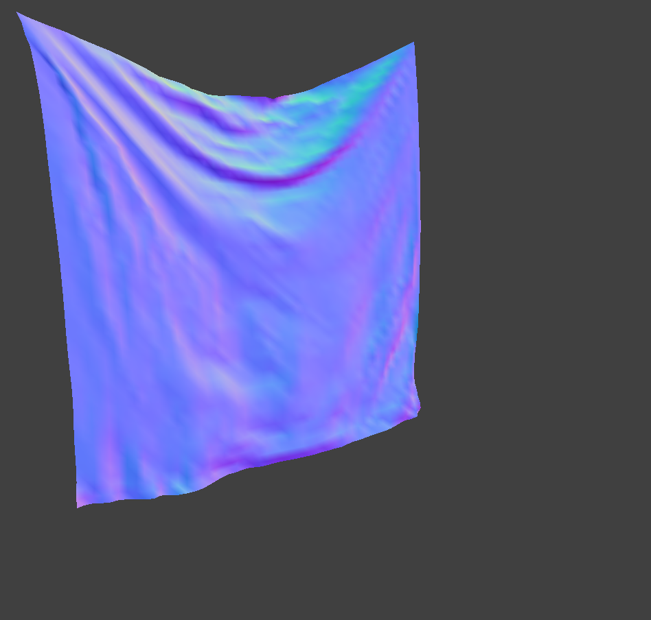
As the results show, a higher Ks (spring constant) results in a tighter cloth surface. Therefore, with a large Ks, the cloth appears flatter and more stretched, while with a smaller Ks, the surface becomes more wrinkled and uneven.
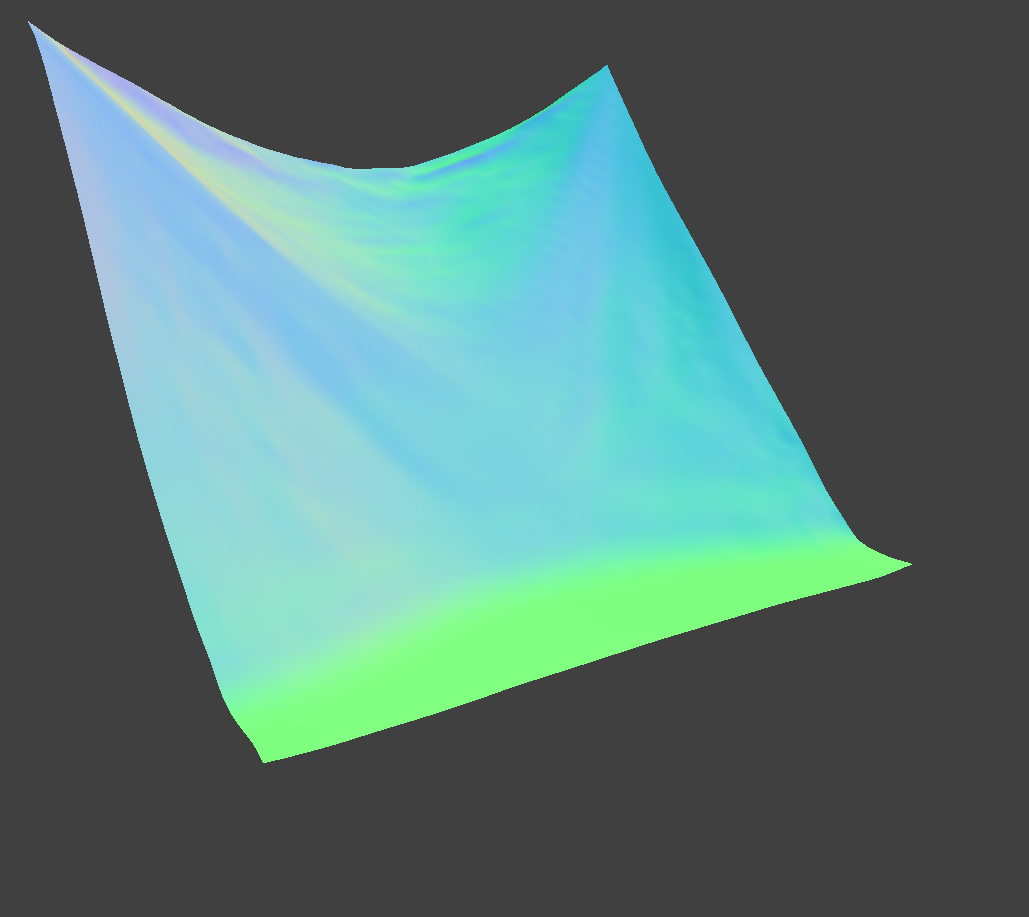
| Default: Ks = 5000 N/m, density = 15 g/cm^2, Damping = 0.2 | ||
|
|
|
|
| Higher Density = 150 g/cm^2 | ||
|
|
|
When the mass of a point mass increases, it effectively weakens the restoring force of the springs. As a result, higher density leads to a more wrinkled cloth surface, while lower density results in a flatter appearance.
| Default: Ks = 5000 N/m, density = 15 g/cm^2, Damping = 0.2 | ||
|
|
|
|
| Higher Damping = 0.5 | ||
|
|
|
A larger damping coefficient means that the cloth responds more slowly to external forces, resulting in a less noticeable increase in velocity compared to a smaller damping value. In the simulation, this manifests as the cloth falling more slowly.
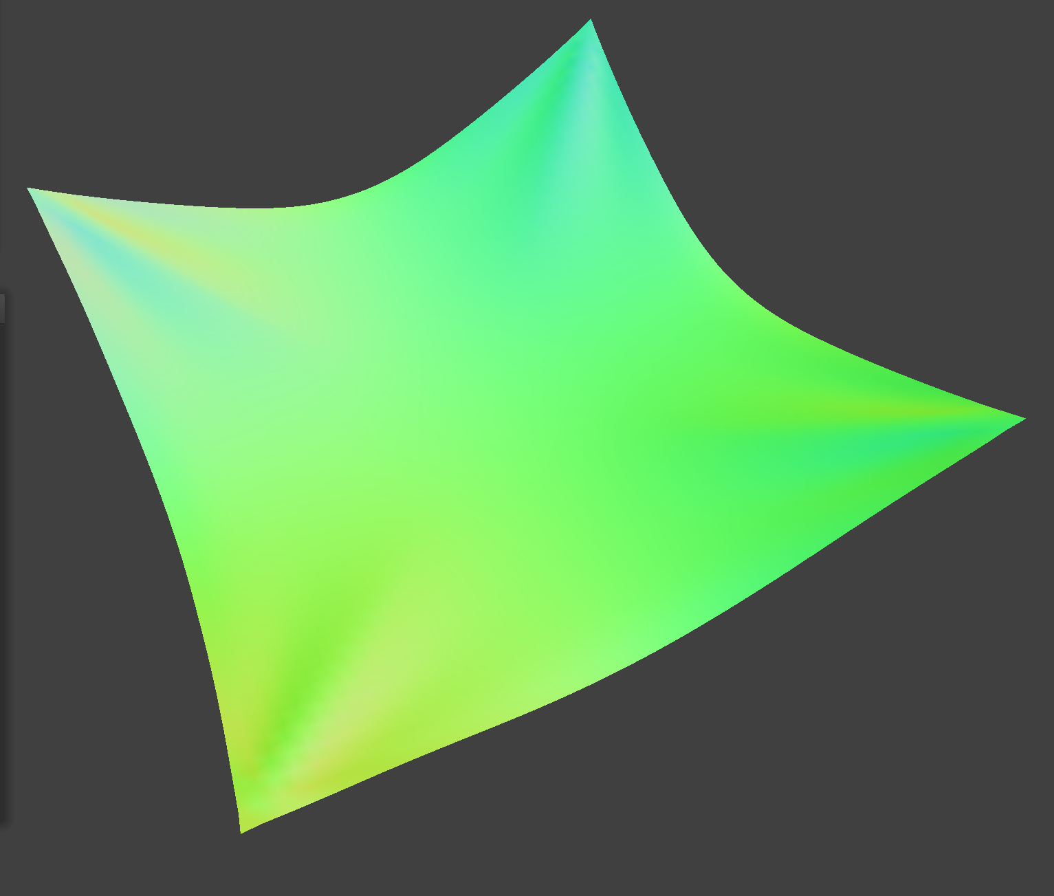
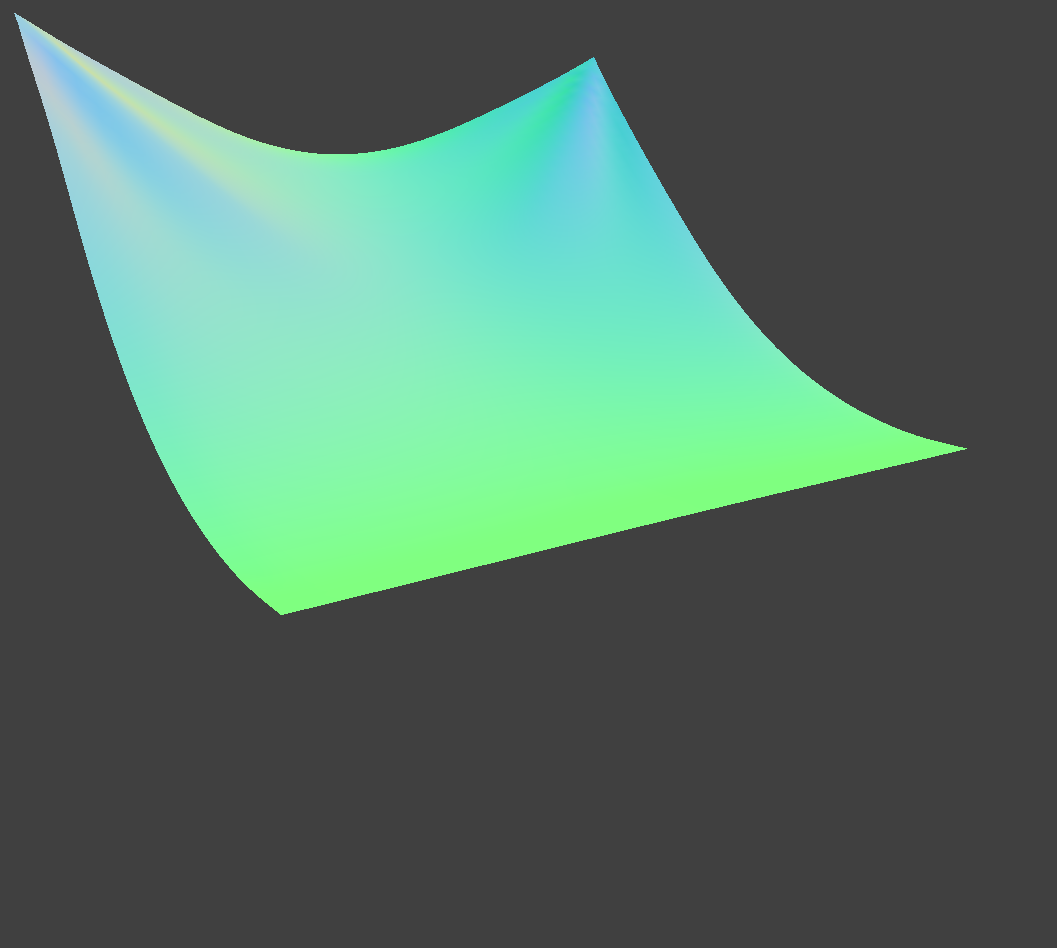
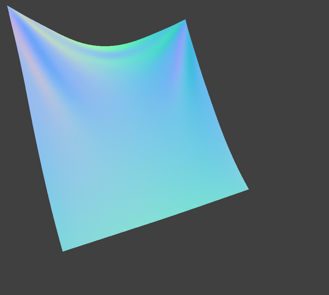
Converged pinned4.json, where four corners of the cloth are pinned.
Part 3: Collisions with Other Objects
Collision with Sphere
- Check whether the point mass pm is colliding with the sphere:
- Compute the distance between the point mass's current position (pm.position) and the sphere's origin;
- If the distance is greater than or equal to the radius, no collision has occurred, so return immediately.
- If a collision is detected, handle it as follows:
- Compute the tangent point on the sphere surface:
- Normalize the vector (pm.position - origin), multiply by the radius;
- Add the sphere origin to get the point on the sphere surface.
- Calculate the correction vector:
- Subtract the previous position pm.last_position from the tangent point.
- Update the current position pm.position:
- Set it to pm.last_position plus (1 - friction) times the correction vector;
- This simulates friction, reducing the velocity after the collision and causing the point to slide along the sphere.
- Compute the tangent point on the sphere surface:
Collision with Plane
- Set up a ray from the previous position to the current position:
- ray_origin = pm.last_position
- ray_direction = unit vector from pm.last_position to pm.position
- t_min = 0
- t_max = length of the displacement vector
- Check if the ray is parallel to the plane:
- If dot(normal, ray_direction) is near zero, the ray is parallel;
- In this case, there is no intersection, so return.
- Compute the intersection point between the ray and the plane:
- Use the plane equation and ray formula to solve for t_intersect:
t_intersect = dot((point - ray_origin), normal) / dot(normal, ray_direction) - If t_intersect is outside [t_min, t_max], the segment doesn’t hit the plane, so return.
- Use the plane equation and ray formula to solve for t_intersect:
- If a collision occurs:
- Calculate the intersection point with a slight offset to prevent
sticking:
intersection_point = ray_origin + ray_direction * (t_intersect - SURFACE_OFFSET)
- Compute the correction vector:
correction_vector = intersection_point - ray_origin
- Update the point mass position:
pm.position = pm.last_position + (1 - friction) * correction_vectorThis simulates a collision response with friction, allowing the cloth to slide along the plane instead of bouncing or sticking unnaturally.
- Calculate the intersection point with a slight offset to prevent
sticking:
Result Gallery
|
|
|
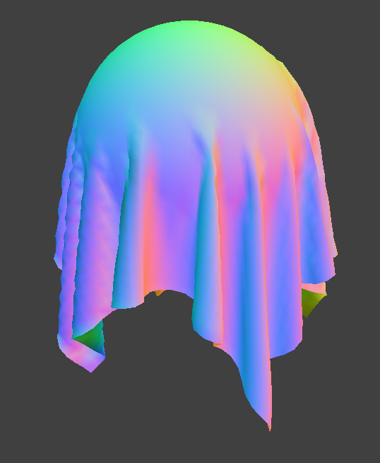
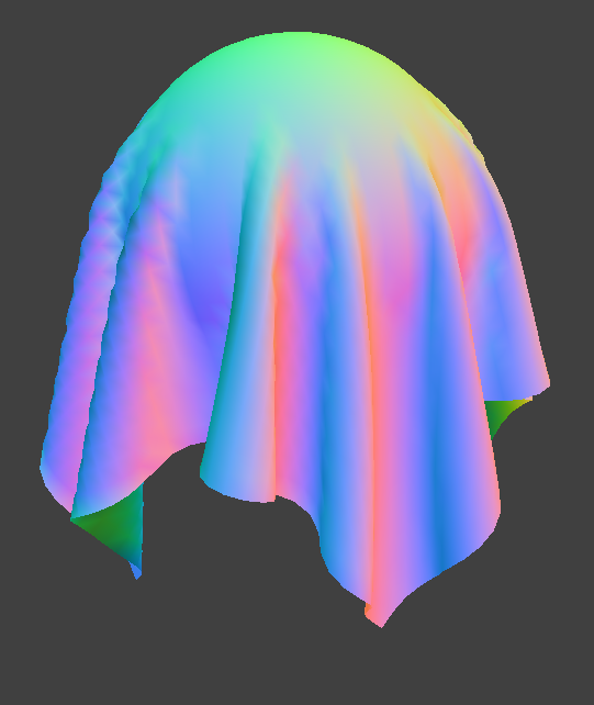
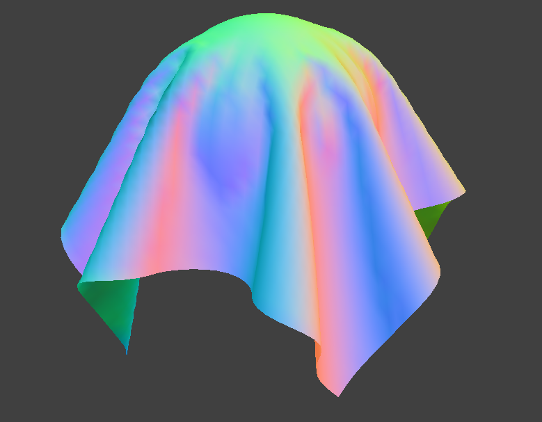
| Cloth Ks = 500 | Cloth Ks = 5000 | Cloth Ks = 50000 |
From the images, we observe that as the spring constant Ks increases, the cloth becomes more resilient and is better able to preserve its original shape, rather than completely draping and conforming to the surface of the sphere.
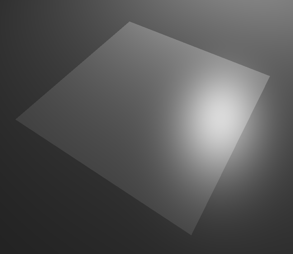
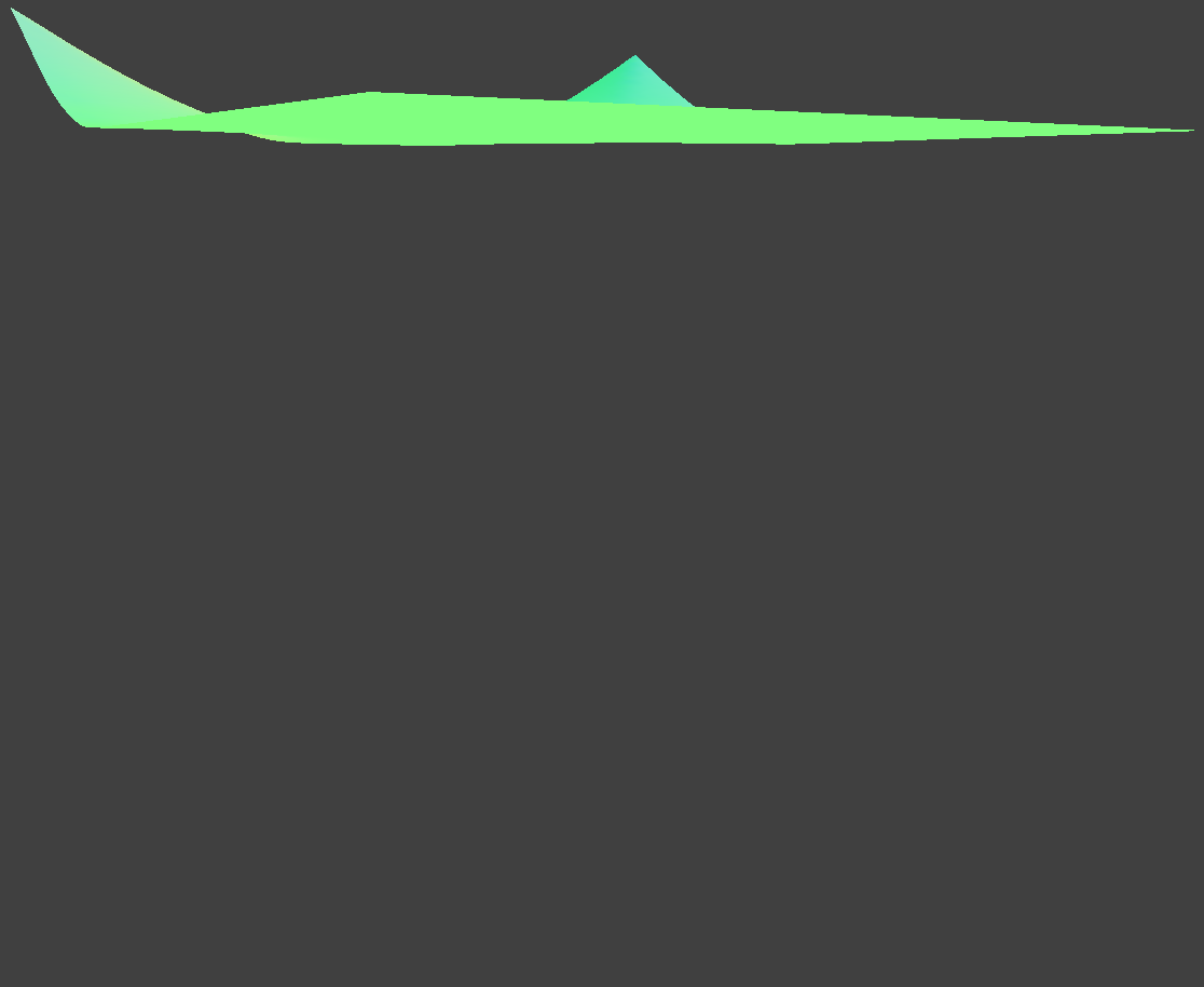
A planar cloth lying restfully on a plane.
Part 4: Self Collision
In each simulation step, we use spatial hashing to find point masses that are neighboring, and test if they collide.
Hashing Spatial Points
Compute grid sizes for each axis:
wis a scaled width bin size based on the cloth resolution.his the height bin size.tis the maximum ofwandhto ensure cubic spacing.
Convert 3D position into discrete grid coordinates (x, y, z) by flooring the position values divided by the bin size.
Combine (x, y, z) using a set of large prime multipliers and XOR operations to generate a unique hash key.
Building Spatial HashMap
- Clear the existing spatial hash map:
- Iterate through all entries in the map and delete their associated vector pointers.
- Clear the map to remove all old entries.
- Rebuild the spatial map for the current point mass positions:
- For each point mass in the cloth:
- Compute its spatial hash using hash_position().
- If the hash key doesn't exist in the map, create a new vector for that bin.
- Add a pointer to the point mass into the appropriate spatial bin.
- For each point mass in the cloth:
Handling Self Collisions
Compute the hash key of the current point mass using its position.
If the hash bin is empty (no nearby particles), return early.
Initialize a correction vector and counter to accumulate collision responses.
For each candidate point mass in the same bin:
- Skip if the candidate is the same as pm.
- Compute the vector direction and distance between pm and the candidate.
- If the distance is less than 2 × thickness (i.e., they are overlapping), compute the separation correction vector and accumulate it.
- Increase the correction count.
If any collisions were found:
- Average the correction vector across all overlaps.
- Scale it by the number of simulation steps to distribute it smoothly.
- Apply the correction to pm’s position.
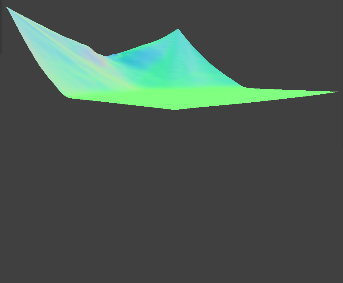
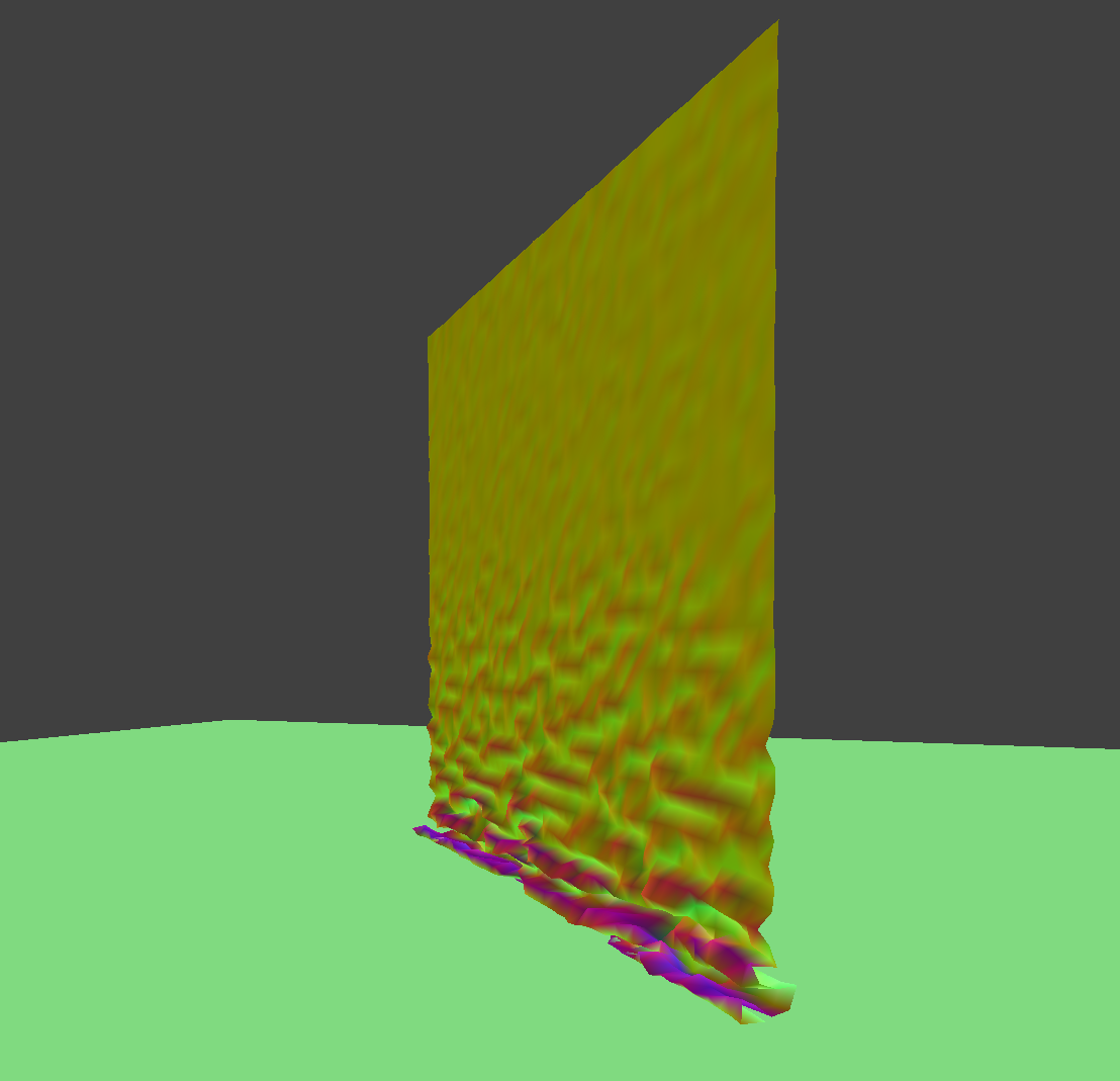
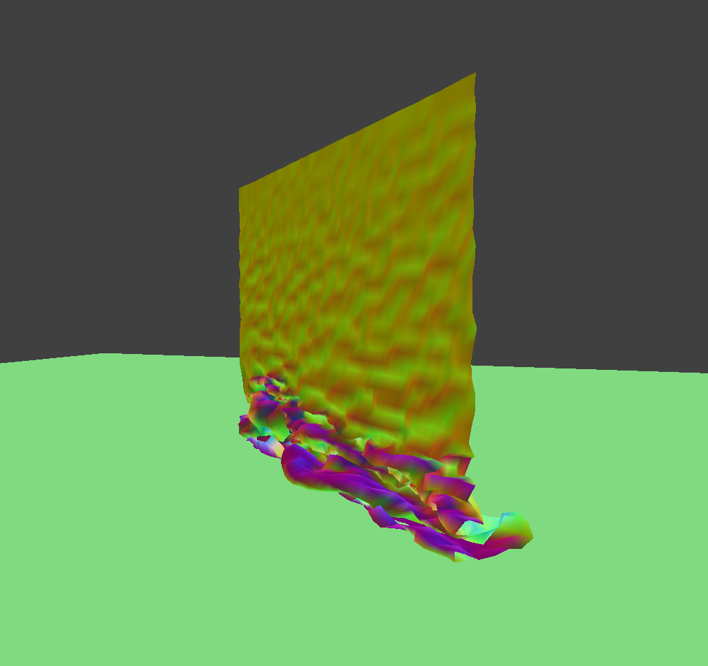
Result Gallery
|
|
|
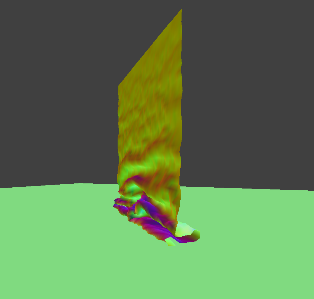
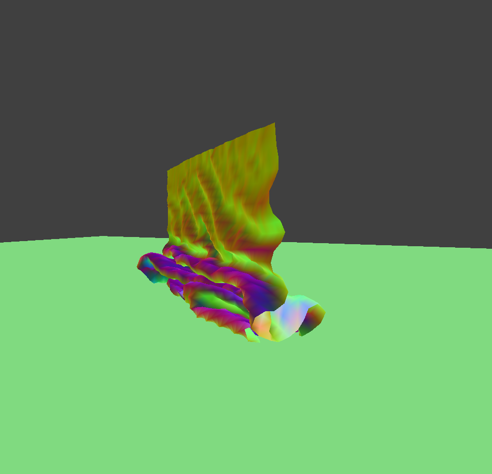
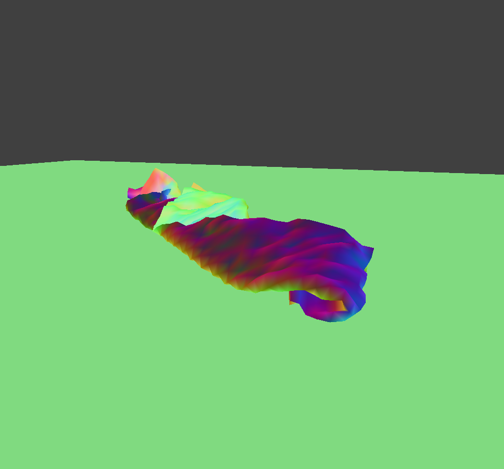
| Falls and folds with default parameters (density = 15, Ks = 5000) | ||
|
|
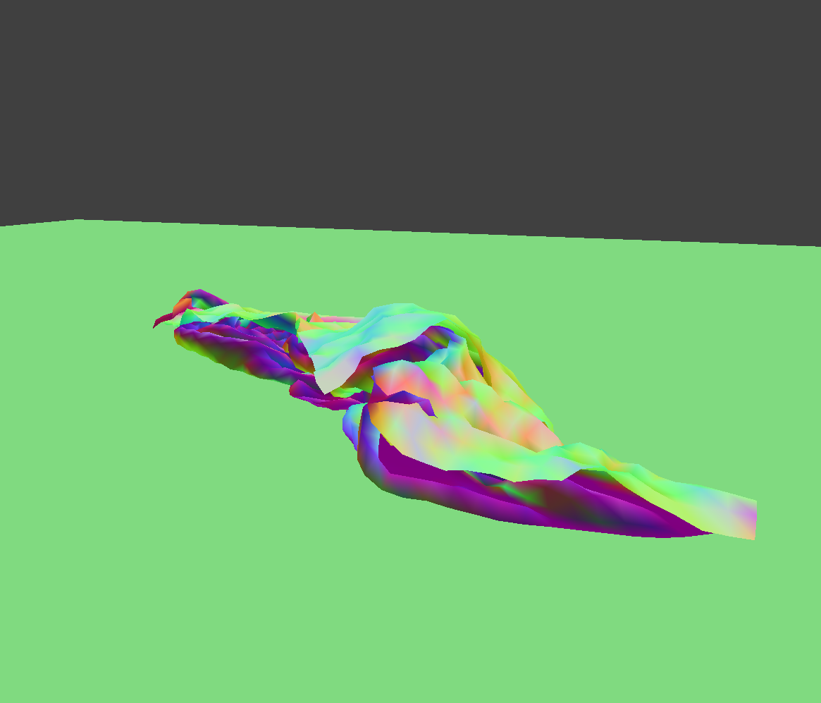
|
| Greater density (d = 150) | ||
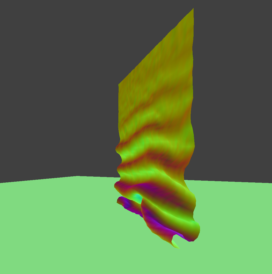
|
|
|
| Greater spring coefficient (Ks = 50000) | ||
The first set of images shows a piece of cloth falling onto itself and experiencing self-collision under normal parameters. In the second set, a higher point mass density is used, resulting in the cloth being compressed more significantly and appearing more tightly packed in its final state. The third set uses a larger spring constant, causing the cloth to better preserve its original shape and appear looser in the final state.
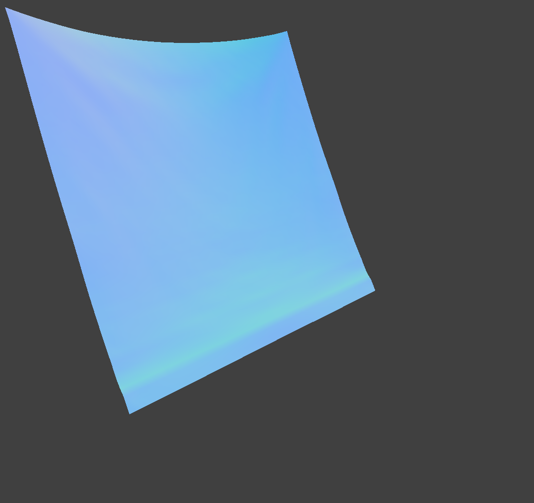
Part 5: Shading
Shaders Introduction
A shader program is a small GPU-executed program used in the rendering pipeline. It consists of multiple shader stages (typically vertex and fragment shaders) and controls how geometry and pixels are processed on screen.
A vertex shader operates on each vertex of a 3D object. It handles transformations (like model-view-projection), computes per-vertex data (such as normals or texture coordinates), and outputs information to the next stage of the pipeline.
A fragment shader runs on each pixel (fragment) generated after rasterization. It determines the final color of a pixel, applying effects such as lighting, texturing, and shading.
Blinn-Phong Shader
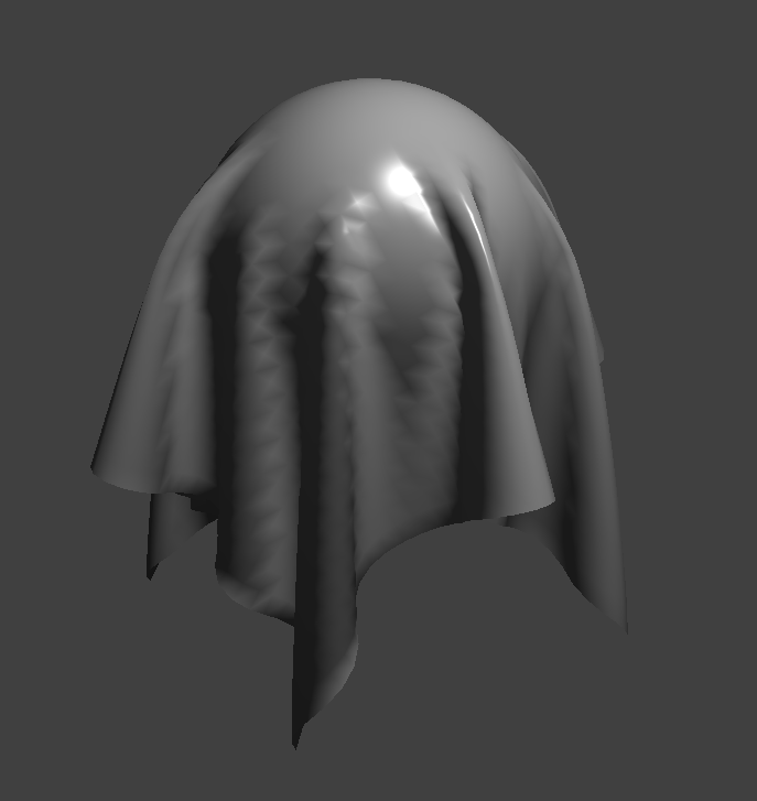
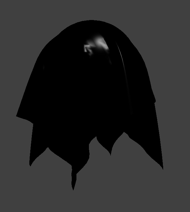
Blinn-Phong shading models consist of three components:
- Ambient component simulates indirect lighting. It adds a constant light to all surfaces, ensuring they are visible even without direct light.
- Diffuse component models light scattered evenly in all directions from a rough surface. It depends on the angle between the light direction and the surface normal.
- Specular component represents shiny highlights caused by direct reflection of light. In Blinn-Phong, it uses the half-vector between the light direction and view direction to calculate the intensity.
|
|
|

|
| Full Blinn-Phong Model | Specular | Diffuse | Ambient |
Texture Shader
For texture models, we use:
- A
uniform sampler2D in_textureas the texture texture()to do sampling in sampling space- Each pixel is shaded as
The result is shown as:
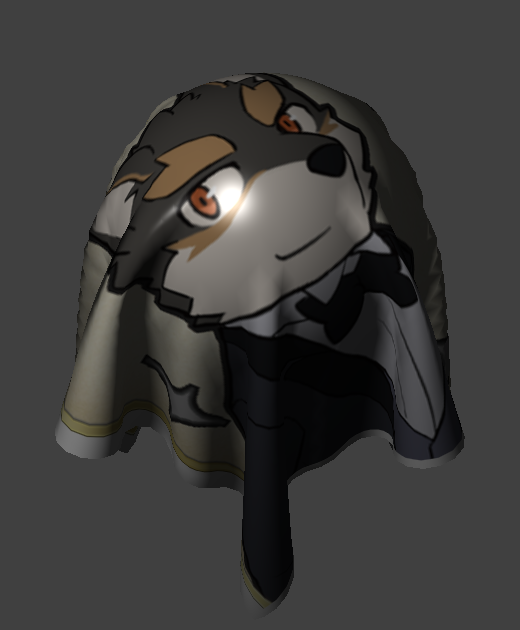
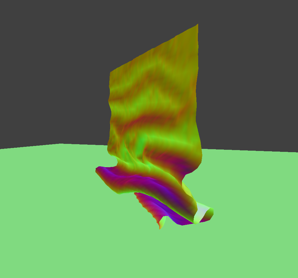
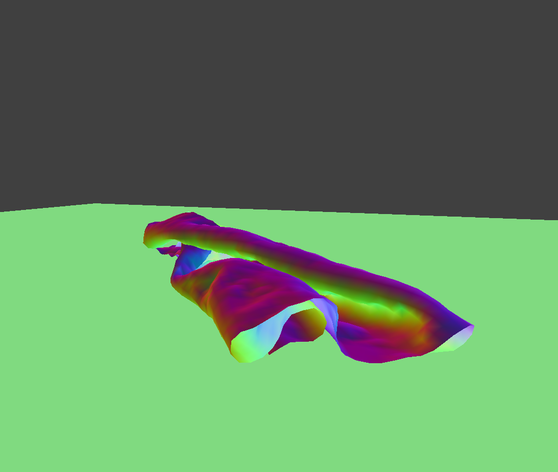
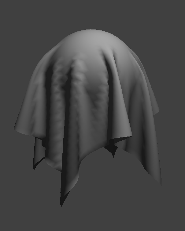
Texture (with Blinn-Phong shading to make it look fine)
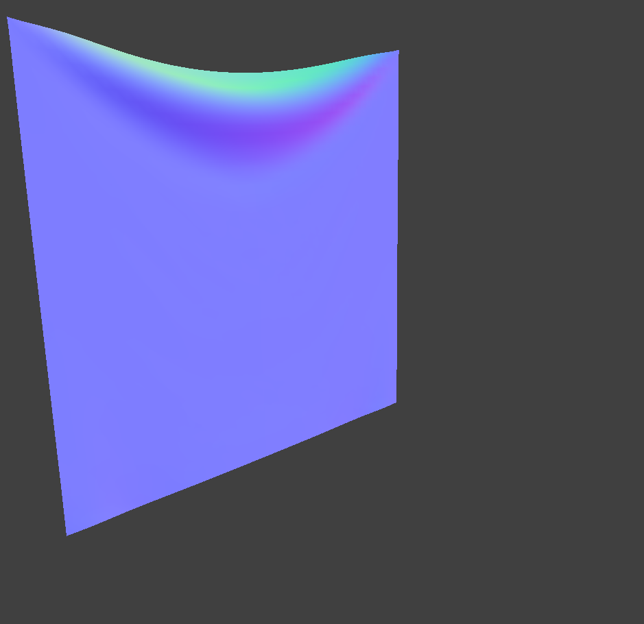
Bump & Displacement Shader
Bump Shader (Frag)
- Construct the TBN matrix (Tangent, Bitangent, Normal):
t: Tangent vector from vertex input, normalized.b: Bitangent is computed as the cross product of normal and tangent.n: Normal vector, normalized.tbn: 3x3 matrix that transforms bump-normal from tangent space to world/view space.
- Compute bump-mapped normal:
- Sample height values h(x, y) from a height function (e.g., texture or procedural).
- Use finite differences in U and V directions to compute slope:
dUis the change in height along the horizontal axis.dVis the change along the vertical axis.- Both are scaled by
u_height_scalingandu_normal_scaling.
- Construct a new tangent-space normal vector
n0 = (-dU, -dV, 1), and normalize it. - Transform
n0using the TBN matrix to get the world/view space normalnd.
- Compute diffuse/specular/ambient lighting (Blinn-Phong model):
- Final output color is the sum of ambient, diffuse, and specular components.
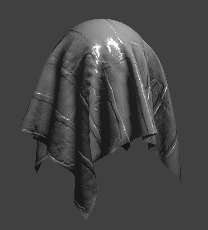
|
|
| Bump Mapping (Default): normal = 2, height = 1 | |
Displacement Shader (Vertex)
- Helper function:
h(uv): Fetches the height value from the red channel of the height map texture at a given UV coordinate.
- Main vertex processing:
- Transform and normalize the vertex normal and tangent using the model matrix.
- Pass UV coordinates unchanged.
- Compute the displaced position:
- Sample the height map at the UV coordinate.
- Scale the normal vector by this height and the user-defined
u_height_scaling. - Add this offset to the model-transformed vertex position to simulate bump displacement.
- Output
gl_Positionby transforming the displaced position with the view-projection matrix.
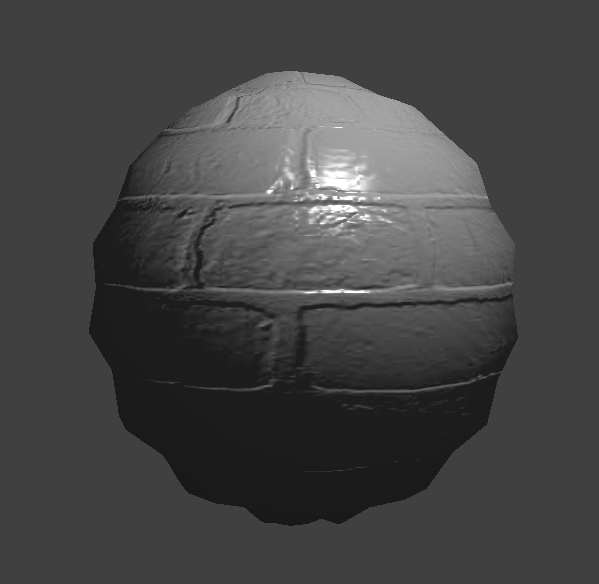
A rendered displacement + bumping shader, setting
normal=100,height=0.02
Comparison
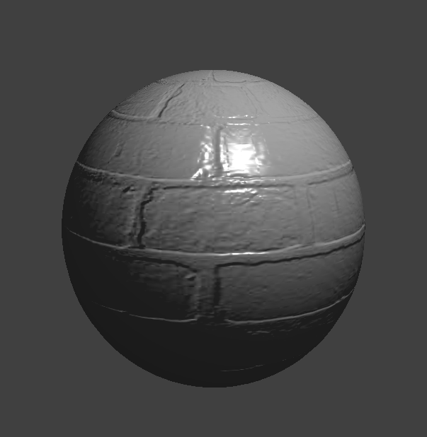
|
|
|
| Bump Mapping | Displacement Mapping |
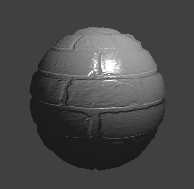
Comparison: Bump mapping doesn't disturb the geometry (vertices), while displacement mapping does. Basically, bump mapping is create an "illusion" of bump by disturbing normals used to render, while displacement mapping actually disturbs the vertex positions. Focus on the outline of the sphere and the differences are clear.
|
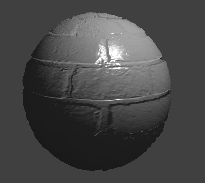
|
| 16 vertices lat/lng direction | 128 vertices lat/lng direction |
With higher number of vertices on the sphere, the displacement mapping works better since it preserves more details of the height disturbance. However, for bump mapping, this doesn't matter since bump mapping don't care vertices.
Environment Mapping
Explanation of mirror mapping fragment shader:
- Compute viewing direction:
view_dir = normalize(u_cam_pos - frag_pos)- This is the direction from the fragment to the camera (eye).
- Compute reflected direction:
refl_dir = reflect(-view_dir, normal)- The incoming view direction is reflected about the surface normal to simulate a mirror-like surface.
- Sample from cube map:
texture(u_texture_cubemap, refl_dir)samples the reflected color from the environment.- This gives the illusion that the surface reflects its surroundings.
- Output:
- The final color (
out_color) is simply the reflected environment color, making the surface look like a perfect mirror.
- The final color (
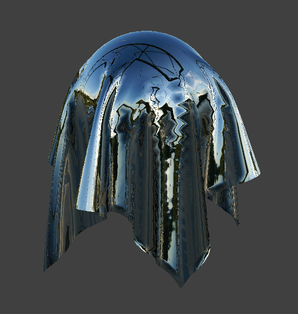
|
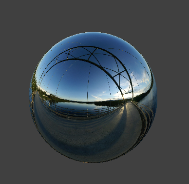
|
| Cloth | Sphere |