My Tiny Path Tracer

Computer Graphics Path Tracing

 2025/03/18 

Overview

This is an implementation of a Path Tracing renderer, with core features of:

BVH Acceleration of Ray-Primitive Intersection
Lambertian BSDF Implementation & Cosine Hemisphere Importance Sampler
Direct Lighting by Importance Sampling Lights
Global Illumination Algorithm
Adaptive Pixel Sampling

Part 1: Ray-Scene Intersection

Ray Generation

First, we generate rays in camera space. We make the following definitions:

Screen Space: $[0, W-1] \times [0, H-1]$
Image Space with Normalized Coordinates: $[0, 1] \times [0, 1]$
Camera Space: $[-\tan(\frac{1}{2}hFoV), \tan(\frac{1}{2}hFoV)] \times [-\tan(\frac{1}{2}vFoV), \tan(\frac{1}{2}vFoV)] \times [-1, 1]$

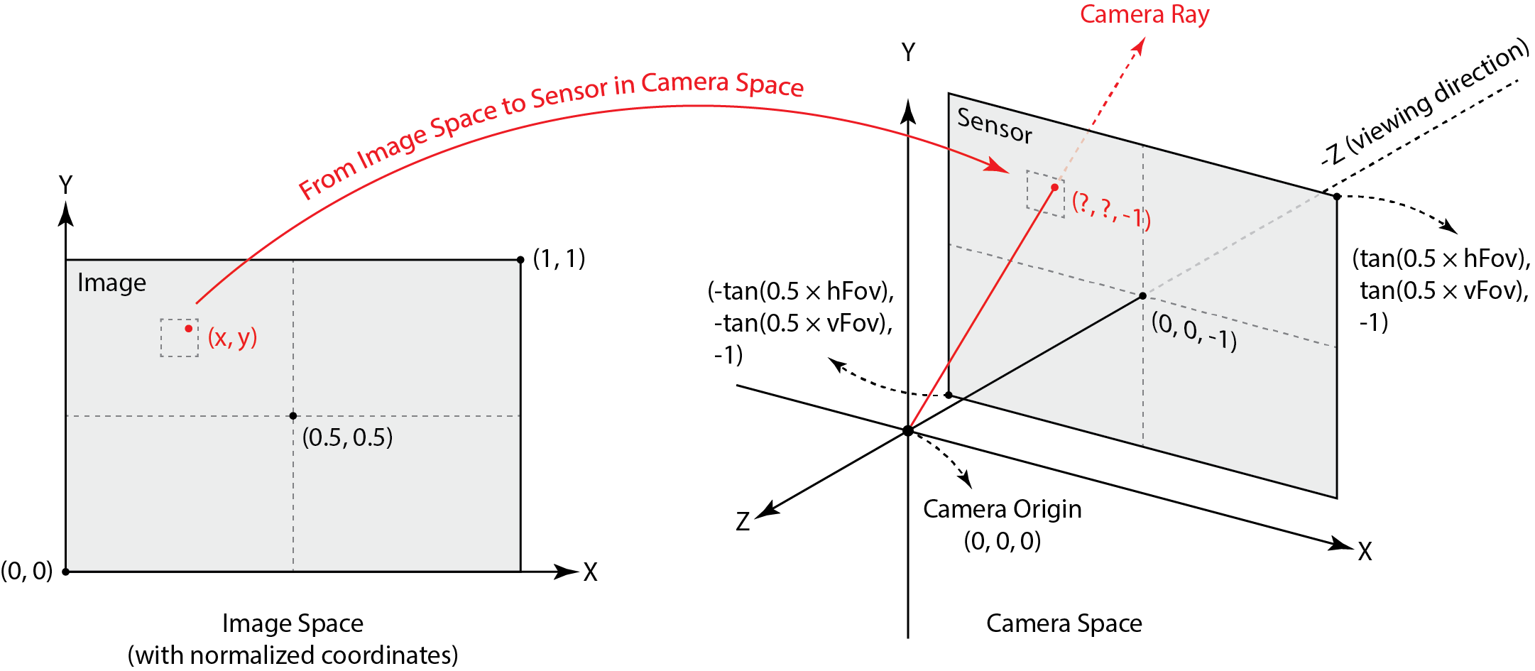
And we generate rays as follows:

Select a pixel $P_{\text{screen}} = [x + rx, y + ry]$ in screen space, where:
- $x \in [0, W-1], y \in [0, H-1]$
- $rx \sim \mathcal{U}(0, 1), ry \sim \mathcal{U}(0, 1)$
Transform $P_{\text{screen}}$ to pixel $P_\text{img}$ in image space, where:
- $P_{\text{img}} = \left[ \frac{P_{\text{screen}}.x}{W}, \frac{P_{\text{screen}}.y}{H} \right]$
Transform $P_\text{img}$ to camera space, where:
- $P_{\text{cam}} = [2\tan(\frac{hFov}{2})( P_{\text{img}}.x - 0.5), \quad2 \tan (\frac{vFoV}{2}) (P_{\text{img}}.y - 0.5), \quad -1]$
Generate ray $r$, where:
- ray.origin = Vector3D(0, 0, 0)
- ray.direction = P_cam.unit()

Ray-Triangle Intersection (3D)

First, we want to know if a ray, defined as $o+td$, has intersection with a plane, defined as $N \cdot (P - P_0) = 0$. The formula is: \[ t = \frac{(\mathbf{P_0} - \mathbf{O}) \cdot \mathbf{N}}{\mathbf{D} \cdot \mathbf{N}} \] Thus if ray.min_t <= t <= ray.max_t, there is an intersection with the plane.

Second, we want to know if the intersection is inside the triangle. This can be verified by barycentric coordinates, which is calculated by formula as follows: \[ p = a v_1 + b v_2 + c v_3 \]

\[ \Rightarrow \begin{cases} p \cdot v_1 = a (v_1 \cdot v_1) + b (v_2 \cdot v_1) + c (v_3 \cdot v_1) \\ p \cdot v_2 = a (v_1 \cdot v_2) + b (v_2 \cdot v_2) + c (v_3 \cdot v_2) \\ p \cdot v_3 = a (v_1 \cdot v_3) + b (v_2 \cdot v_3) + c (v_3 \cdot v_3) \end{cases} \]

This is: \[ \begin{bmatrix} v_1 \cdot v_1 & v_2 \cdot v_1 & v_3 \cdot v_1 \\ v_1 \cdot v_2 & v_2 \cdot v_2 & v_3 \cdot v_2 \\ v_1 \cdot v_3 & v_2 \cdot v_3 & v_3 \cdot v_3 \end{bmatrix} \begin{bmatrix} a \\ b \\ c \end{bmatrix} = \begin{bmatrix} p \cdot v_1 \\ p \cdot v_2 \\ p \cdot v_3 \end{bmatrix} \] Which has a closed form solution. If $0 \le a, b, c \le 1$, the intersection on the plane is in the triangle.

Remark: This method avoids calculating determinant of triangle, which may introduce det=0 cases and needs special if branches. Hence, this method is more effective and numerically stable. (The left 3x3 matrix is always invertible.)

Ray-Sphere Intersection (3D)

Suppose our ray is defined as $o+td$, while sphere is defined as $\| P - c \|^2 = r^2$. The intersection formula is: \[ \begin{cases} t_1 = \frac{-b - \sqrt{\Delta}}{2a} \quad \text{(smaller intersection)} \\ t_2 = \frac{-b + \sqrt{\Delta}}{2a} \quad \text{(larger intersection)} \end{cases} \] where: \[ \begin{cases} a = \|\mathbf{d}\|^2 \\ b = 2 (\mathbf{o} - \mathbf{c}) \cdot \mathbf{d} \\ c = \| \mathbf{o} - \mathbf{c} \|^2 - r^2 \\ \Delta = b^2 - 4ac \end{cases} \] Hence if (ray.min_t <= t1 <= ray.max_t) || (ray.min_t <= t2 <= ray.max_t), there is intersection. And we always take the smaller intersection point.

Result Gallery

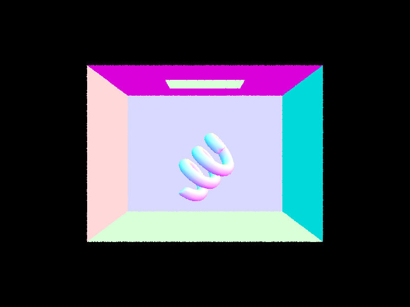
A coil inside a Cornell Box, rendered with normal shading.

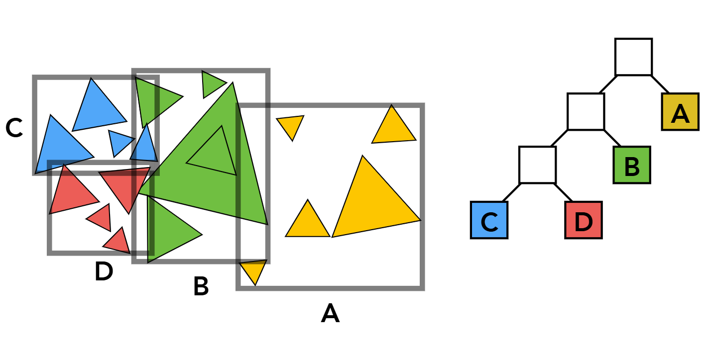
Part 2: Bounding Volume Hierarchy

Default rendering process requires ray-primitive intersection test for each primitive and each ray. Suppose we have $R$ rays and $P$ primitives, this is $\mathcal{O}(R*P)$ complexity. To speed it up, we build hierarchy in primitives and reduce the complexity to $\mathcal{O} (R * \log P)$.

Building BVH Node

The algorithm is as follows:

Function Construct_BVH builds BVH Node of all primitives in [start, end).
Requires primitive iterator start, end; integer max_leaf_size:
Initialize current BVH Node node using a bounding box of all primitives in primitive[start, end].
Check if we need to stop constructing. If end - start <= max_leaf_size:
1. Let node->start = start, node->end = end.
2. Return node.

Otherwise, we want to keep splitting.

First, select pivot using heuristic pivot_axis = argmax(bbox.extent).

Second, we divide the vector into left & right subparts, while the pivot element is the median value on pivot_axis.

auto comp = [&pivot_axis](const Primitive* a, const Primitive* b)
  { return a->get_bbox().centroid()[pivot_axis] < 
           b->get_bbox().centroid()[pivot_axis]; };
auto pivot_pos = start + (end - start) / 2;
std::nth_element(start, pivot_pos, end, comp);

Generate left & right nodes recursively, i.e.

1 2	node->l = construct_bvh(start, pivot_pos + 1, max_leaf_size); node->r = construct_bvh(pivot_pos + 1, end, max_leaf_size);

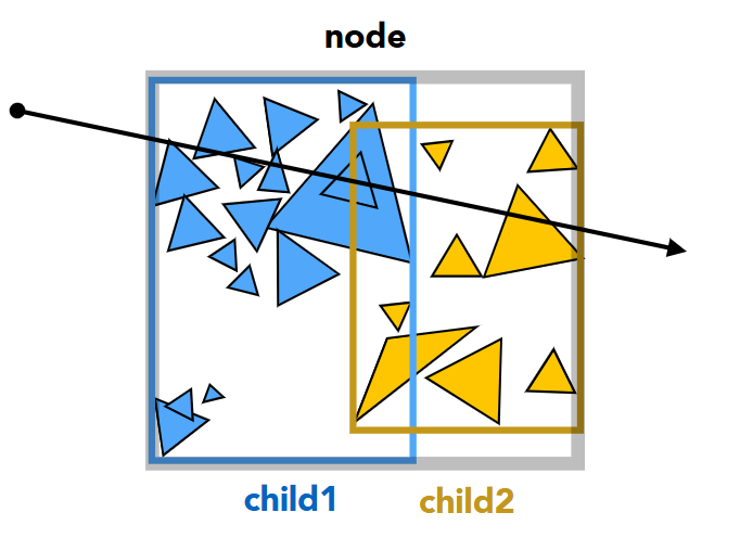
Ray-BVH Intersection

The algorithm is as follows:

Function intersect tests whether a given ray intersects any primitive within a BVH node.
Requires ray (input ray), i (pointer to intersection record), node (current BVH node).
Compute the intersection of the ray with the node's bounding box.
1. Initialize temp_tmin, temp_tmax for storing intersection intervals.
2. If the ray does not intersect the bounding box, return false.
If node is not a leaf, we must check both child nodes.
1. Recursively test intersection with the left child node.
2. Recursively test intersection with the right child node.
3. Return true if either child node is hit.
Otherwise, if node is a leaf, we must check individual primitives.
1. Iterate through all primitives in [node->start, node->end).
2. For each primitive:
  - Increase total_isects (for counting intersections).
  - Update hit if an intersection occurs.
3. Return hit, indicating whether the ray intersects any primitive in the leaf node.

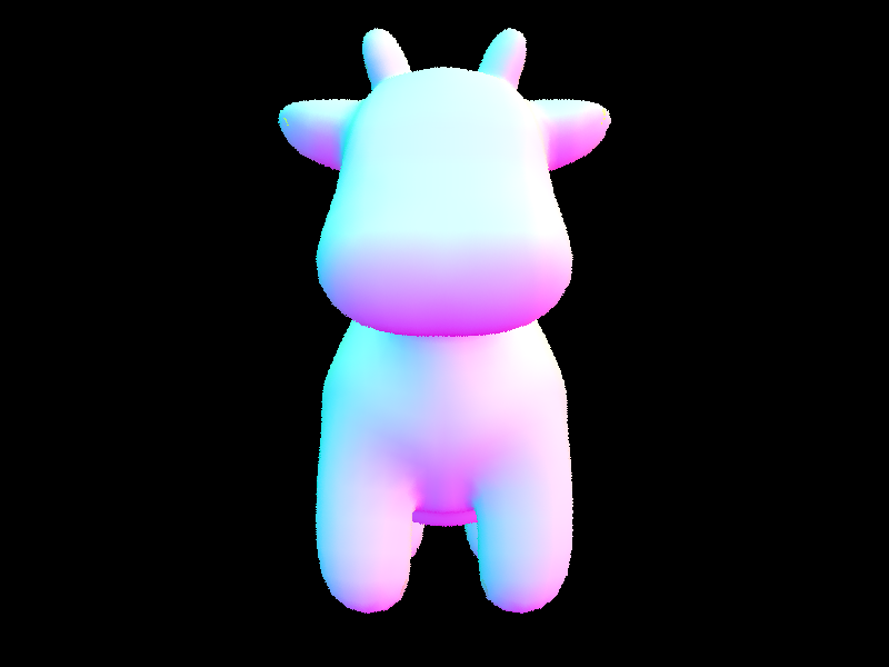
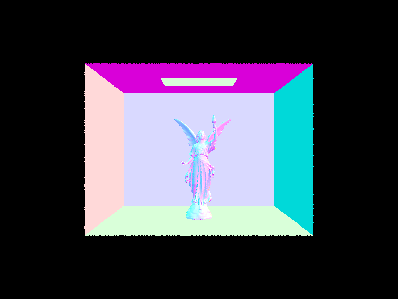
Result Gallery

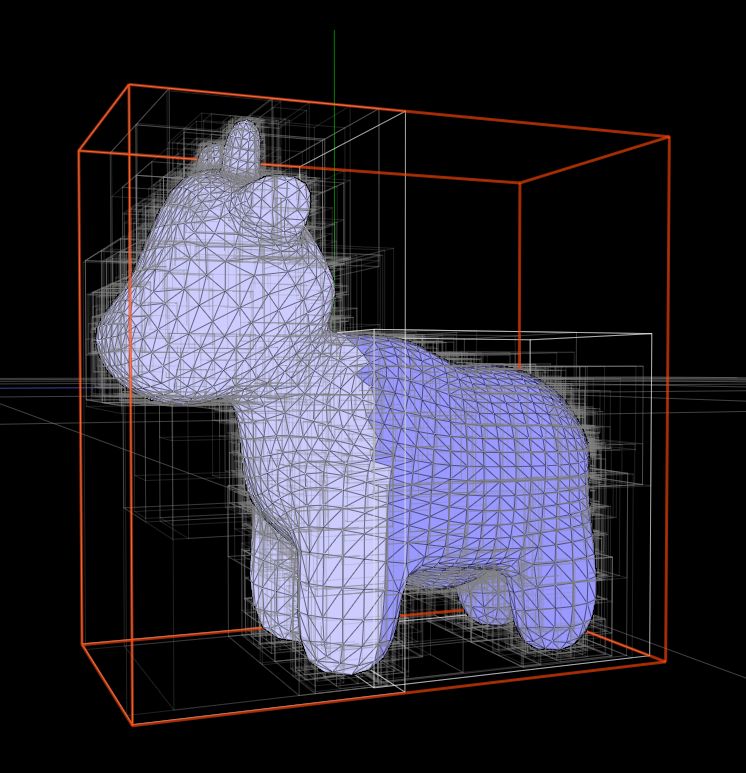
A cow, divided into BVH nodes.

A cow (left) and a lucy statue in a Cornell Box (right), rendered with BVH acceleration and normal shading.

	BVH	Vallina	#Primitives	Rel. Speed
cow	0.1823s	21.1210s	5856 faces	115.85x faster
lucy	0.2515s	826.8349s	133796 faces	3287.6139x faster

Performance comparison. As we can see, with more #primitives, the difference in rendering time is bigger, due to the $\log$ difference in algorithm complexity. For image lucy, it is almost not intractable to render without BVH acceleration, since our current renderer hasn't introduced lighting yet.

Part 3: Direct Illumination

The Lambertian BSDF

We will derive the Lambertian reflectance BSDF, which is a uniform matte texture, as follows:

We assume that the BSDF $f_r(p, w_i \rightarrow w_o)$ is constant $C$ for all incident and outgoing directions.
The outgoing radiance at a point $p$ in direction direction $\omega_o$ is given by the reflection equation: \[ L_r(p, \omega_o) = \int_{H^2} f_r(p, \omega_i \to \omega_o) L_i(p, \omega_i) \cos\theta_i d\omega_i \] Since we assume that $f_r$ is constant, we can take it out of the integral: \[ L_r(p, \omega_o) = f_r \int_{H^2} L_i(p, \omega_i) \cos\theta_i d\omega_i \] The integral represents the irradiance $E_i$ at $p$, so we rewrite it as: \[ L_r(p, \omega_o) = f_r E_i \]
By the definition of reflectance (also called albedo), the fraction of incident energy that is reflected is: \[ \frac{L_r(p, \omega_o)}{E_i} = \text{Reflectance} \] Substituting $L_r(p, \omega_o) = f_r E_i$, we have: \[ f_r = \frac{\text{Reflectance}}{\pi} \] This is the BSDF of Lambertian reflectance model.

Direct Lighting Calculation (Hemisphere Sampling)

The algorithm is as follows:

Function estimate_direct_lighting_hemisphere estimates direct lighting at an intersection point using hemisphere sampling.
- Requires: Ray r, Intersection isect.
- Returns: Estimated direct lighting L_out.
Construct a Local Coordinate System
- Align the normal $N$ of the intersection point with the Z-axis.
- Compute the object-to-world transformation matrix o2w and its transpose w2o.
- Define w_in_objspace, w_out_objspace, w_in_world, w_out_world
Sample the Hemisphere
- Set number of samples proportional to the number of scene lights and area light samples.
- For each sample:
  1. Sample the BSDF to generate an incoming direction w_in_objspace and its pdf.
  2. Construct a shadow ray from the hit point along the sampled direction.
  3. Check for occlusion:
    - If the shadow ray hits another object, retrieve the emitted radiance $L_{\text{in}}$.
    - Accumulate contribution: \[ L_{\text{out}} := L_{\text{out}} + f_r \cdot L_{\text{in}} \cdot \cos\theta / \text{pdf} \]
Normalize by Sample Count by dividing L_out by the total number of samples.
Return the Estimated Radiance L_out.

Result Gallery: Uniform Hemisphere Sampling


#samples/light ray: 1	#samples/light ray: 4	#samples/light ray: 16	#samples/light ray: 64

Importance Sampling on Lambertian Materials

We will prove that using cosine sampling on Lambertian Materials is better than uniform sampling.

Monte Carlo Integration Variance Formula:
\[ \text{Var}(I) = \frac{1}{N} \text{Var} \left(\frac{f}{p} \right) \] where $ f $ is the function and $ p $ is the sampling PDF.
For Uniform Sampling:
- The PDF $p = \frac{1}{\pi}$ (uniform over the hemisphere).
- The function to integrate: \[ f = \text{reflectance} \cdot \cos\theta \].
- Importance ratio:
  \[ \frac{f}{p} = 2 \cdot \text{reflectance} \cdot \cos\theta \]
- Variance is nonzero due to $\cos\theta$ fluctuations.
For Cosine Sampling:
- The PDF $ p = $ (proportional to Lambertian reflectance).
- Importance ratio:
  \[ \frac{f}{p} = \text{reflectance} \]
- Variance is zero because $ f/p $ is constant.
Conclusion:
- Cosine-weighted sampling perfectly cancels out the $ $ term, reducing variance to zero.
- Uniform sampling has unnecessary variance, making it less efficient for rendering Lambertian surfaces.
- Cosine sampling converges faster with fewer samples, improving efficiency in Monte Carlo integration.

Difference in code implementation of DiffuseBSDF::sample_f

Uniform Sampling:

1
2
3

*wi = UniformHemisphereSampler3D().get_sample();
*pdf = 1 / (2 * PI);
return f(wo, *wi) * 2 * cos_theta(*wi);

Cosine Sampling:

1
2
3

*wi = CosineWeightedHemisphereSampler3D().get_sample();
*pdf = cos_theta(*wi) / PI;
return f(wo, *wi);

Direct Lighting Calculation (Importance Sampling)

The algorithm is as follows:

Function estimate_direct_lighting_importance estimates direct lighting at an intersection point using importance sampling.
- Requires: Ray r, Intersection isect.
- Returns: Estimated direct lighting L_out.
Construct a Local Coordinate System... (omitted, same as above.)
Sample the Lights Using Importance Sampling
- Iterate over all light sources in the scene.
- For each light:
  1. Sample the light source to generate an incoming direction w_in_world, its pdf, and the emitted radiance $ L_{} $.
  2. Transform w_in_world into object space to get w_in_objspace.
  3. Construct a shadow ray from the hit point along the sampled direction.
  4. Check for occlusion:
    - If the shadow ray does not hit an occluder:
      - Compute the BSDF value $ f_r $.
      - Accumulate contribution: \[ L_{\text{out}} := L_{\text{out}} + f_r \cdot L_{\text{in}} \cdot \cos\theta / \text{pdf} \]
Return the Estimated Radiance L_out

Result Gallery: Importance Sampling

Hemisphere Sampling

#samples/light ray: 1	#samples/light ray: 4	#samples/light ray: 16	#samples/light ray: 64
Importance Sampling

#samples/light ray: 1	#samples/light ray: 4	#samples/light ray: 16	#samples/light ray: 64

In comparison, using importance sampling makes convergence much faster than direct uniform sampling. Even if we only sample ONCE per light ray, importance sampling can still generate reasonable results, while uniform sampling can almost see nothing in the image. Remark: we use one sample per pixel for all results here.

Part 4: Global Illumination

Recursive Path Tracing (Fixed N-Bounces)

The algorithm is as follows:

Function at_least_one_bounce_radiance_nbounce computes radiance at an intersection by recursively tracing multiple bounces.
- Requires: Ray r, Intersection isect.
- Returns: Estimated radiance L_out.
Check for Maximum Depth
- If r.depth >= max_ray_depth, return the one-bounce radiance and terminate recursion.
Construct a Local Coordinate System... (omitted, same as above)
Sample the BSDF to Generate a New Ray
- Sample an incoming direction w_in_objspace using the BSDF and compute its probability density (pdf).
- Construct a new ray r_new from the intersection point along w_in_wspace, with an incremented depth.
Check for Intersection with the New Ray
- If r_new does not hit any object, return one-bounce radiance and terminate recursion.
Compute Radiance Based on Bounce Accumulation Mode
- If isAccumBounces is enabled:
  - Return one-bounce radiance plus recursively computed indirect radiance if depth limit is not reached.
- Otherwise (only indirect light contribution):
  - Return only the recursively computed indirect radiance beyond the first bounce.
Final Radiance Contribution
- The accumulated radiance is computed as: \[ L_{\text{out}} := f_r \cdot L_{\text{rec}} \cdot \cos\theta / \text{pdf} \]
- If isAccumBounces is enabled, direct illumination is added; otherwise, only indirect illumination is computed.
Return the Estimated Radiance L_out

Recursive Path Tracing (Russian Roulette Termination)

The algorithm is as follows:

Function at_least_one_bounce_radiance_rr computes radiance at an intersection using Russian Roulette termination for efficiency.
- Requires: Ray r, Intersection isect.
- Returns: Estimated radiance L_out.
Apply Russian Roulette Termination
- With probability $ 1 - P_{} $, terminate recursion and return one-bounce radiance.
Construct a Local Coordinate System... (omitted, same as above)
Sample the BSDF to Generate a New Ray... (omitted, same as above)
Check for Intersection with the New Ray... (omitted, same as above)
Compute Radiance Based on Bounce Accumulation Mode... (omitted, same as above)
Final Radiance Contribution
- The accumulated radiance is computed as: \[ L_{\text{out}} := f_r \cdot L_{\text{rec}} \cdot \cos\theta / (\text{pdf} \cdot P_{\text{RR}}) \]
- Russian Roulette termination ensures that only a subset of paths continue, but the contribution is unbiasedly scaled by dividing by $ P_{} $.
Return the Estimated Radiance L_out

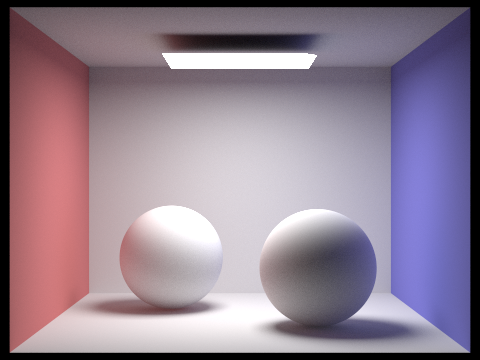
Result Gallery

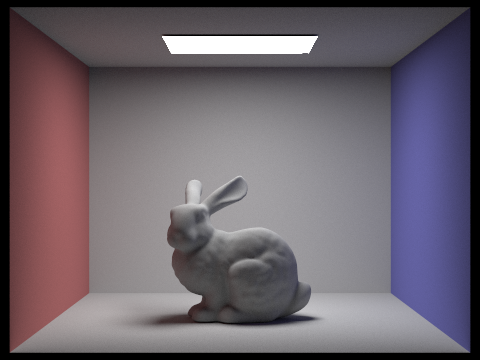
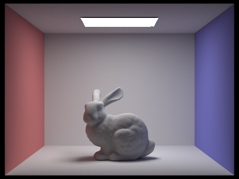
Some images, rendered with global illumination.
1024 samples / pixel, 4 samples / light ray, 5 bounces maximum.

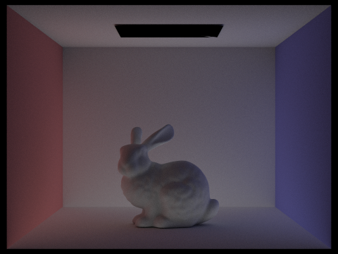
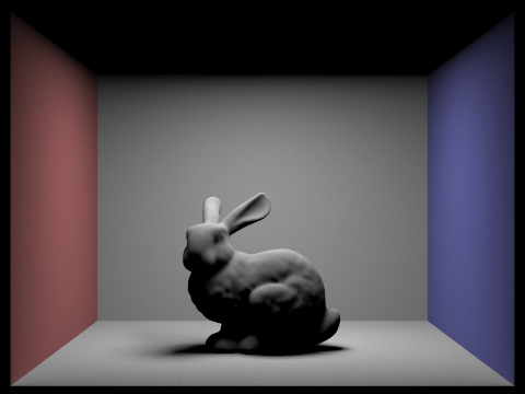
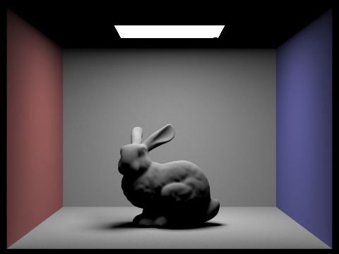
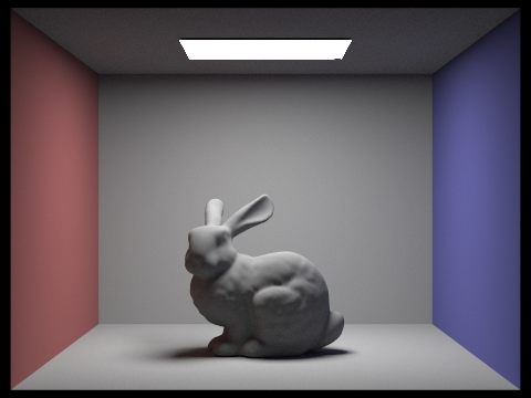
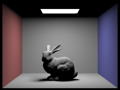
The bunny rendered with only direct lighting (left) and only indirect lighting (right)

Global Illumination

nbounce = 0	nbounce = 1	nbounce = 2	nbounce = 3	nbounce = 4	nbounce = 5
Cumulative Global Illumination

nbounce = 0	nbounce = 1	nbounce = 2	nbounce = 3	nbounce = 4	nbounce = 5

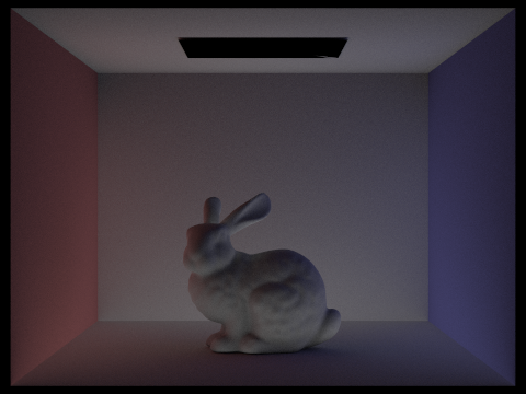
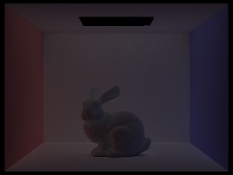
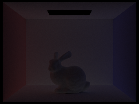
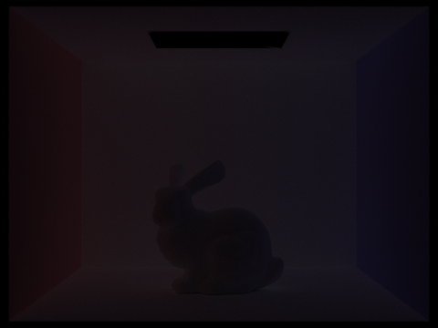
The bunny rendered with mth bounces of light.
1024 samples per pixel, 4 samples per light, nbounces listed in the table.
As we can see, nbounce=2 contributes the "soft shadow" part, where the bottom part of the bunny is lit due to indirect lighting. Also, the left and right side has some red and blue separately, due to indirect lighting from both walls. As comparison, contribution from nbounce >= 3 is not very big afterwards. The box just look slightly brighter on corners, while more red/blue are emitted onto white surfaces.

Russian Roulette (p=0.4)

max_bounce = 0	max_bounce = 1	max_bounce = 2	max_bounce = 3	max_bounce = 4	max_bounce = 100

The bunny, rendered with Russian roulette.
1024 samples per pixel, 4 samples per light, nbounces listed in the table.


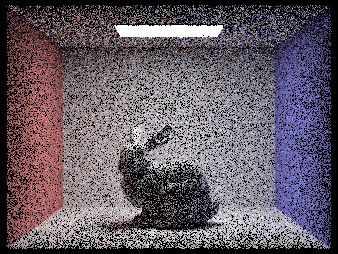
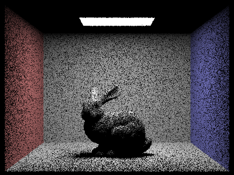
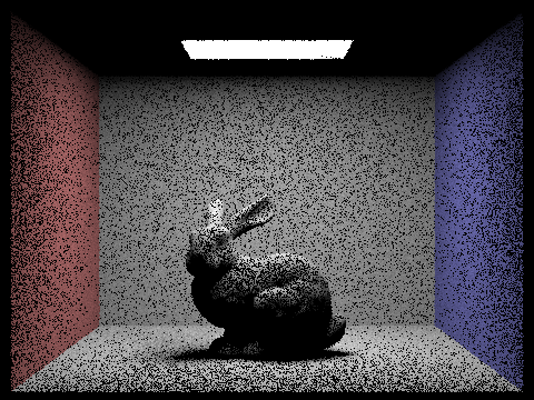
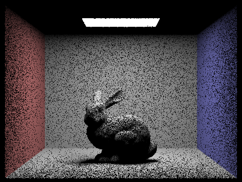
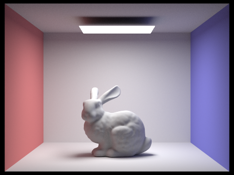
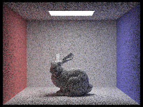
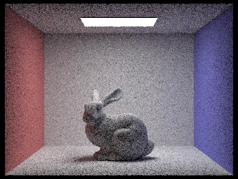
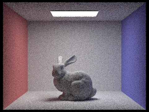
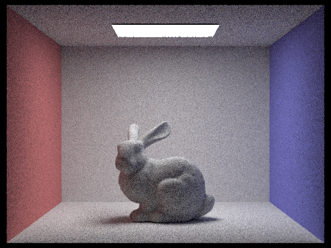
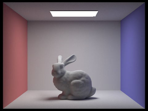
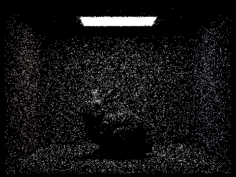
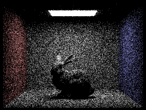
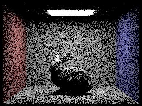
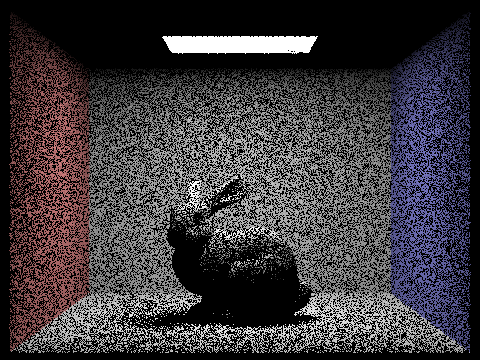
1 s/p	2 s/p	4 s/p	8 s/p	16 s/p	64 s/p	1024 s/p

The bunny, rendered with different #samples/pixel. We use 4 samples/ray, nbounces=5.

Part 5: Adaptive Sampling

Adaptive Sampling Algorithm

We use adaptive sampling to boost efficiency, and reduce the noise in the rendered image. The algorithm is as follows:

Function raytrace_pixel_adaptive adaptively samples a pixel to achieve convergence efficiently.
- Requires: Pixel coordinates (x, y), max samples ns_aa, convergence threshold maxTolerance.
- Returns: Final color for the pixel.
Initialize Sampling Variables
- Set num_samples to the maximum allowed samples.
- Define s1 and s2 to track the sum and squared sum of luminance values.
- Set sample_count = 0 for tracking the actual number of samples taken.
- Initialize color for accumulating radiance estimates.
Iterative Sampling Process
- For each sample:
  1. Estimate radiance using est_radiance_global_illumination(ray).
  2. Accumulate the sampled radiance into color.
  3. Compute the luminance of the sample and update s1 and s2.
  4. Increment sample_count.
Check for Convergence
- Every samplesPerBatch iterations:
  1. Compute the mean luminance:
    \[ \mu = \frac{s1}{\text{sample_count}} \]
  2. Compute the variance:
    \[ \sigma^2 = \frac{s2 - \frac{s1^2}{\text{sample_count}}}{\text{sample_count} - 1} \]
  3. Compute the confidence interval width:
    \[ I = \frac{1.96 \cdot \sigma}{\sqrt{\text{sample_count}}} \]
  4. If $I \leq \text{maxTolerance} \cdot \mu$, stop sampling (pixel has converged).
Normalize the Final Color: Divide color by sample_count to get the final pixel value.
Update Buffers
- Store the final pixel color in sampleBuffer.
- Store the actual number of samples taken in sampleCountBuffer.

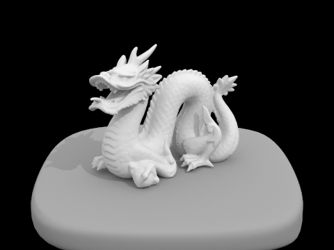
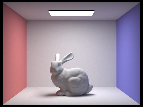
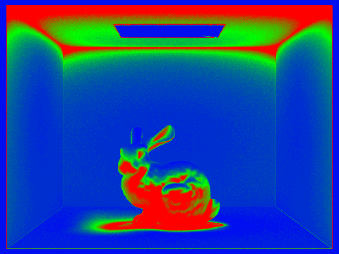
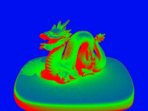
Result Gallery

The bunny (up) and dragon (down) rendered by adaptive sampling. The second column indicates sampling density, where red=higher, green=mdeium, blue=lowest. We use 2048 samples/pixel, 4 samples/ray, nbounces=5.

Author：SimonXie2004

Link：https://simonxie2004.github.io/2025/03/18/Path-Tracer/

Publish date：March 18th 2025, 11:40:48 pm

Update date：March 26th 2025, 5:56:49 am

License：CC-4.0

Previous Post

Re-Inventing VAE on a Retrospective Perspective

CATALOG