
With the Variational AutoEncoders being honored with the ICLR 2024 Time Tested Award, it is a fitting moment to reflect on its journey.
As a groundbreaking idea, VAE has laid solid foundation for Probabilistic Modeling and Generative Models. It shattered the modern belief that deep learning is merely about designing loss functions and NN architectures. Instead, it introduced a probabilistic perspective, emphasizing learning distributions first and transforming objectives into intractable losses.
This is a teaser.
Traditional Compression Models
Traditional lostless compression models like LDA/PCA, come with a price: their latent space are less explainable, and lack useful structures. For example, image manifold need not to be combined from orthogonal base vectors, but PCA is forced to learn an orthogonal one.
Traditional Autoencoders
Traditional autoencoders are basically trying to solve the problem that PCA/LDAs' latent space are too "structered" (e.g. to be orthorgonal.) This is where neural networks come in:
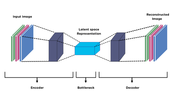
Neural Network: Just like UNet, without skipping connections. Recon-loss: \(\|out - in\|_2^2\)
Problem:
- How to sample from latent space? You don't have \(p_\theta(z)\).
- The model is limited-responsive to some inputs, i.e. interpolating
new z in latent space and decoding it won't generate meaningful image!
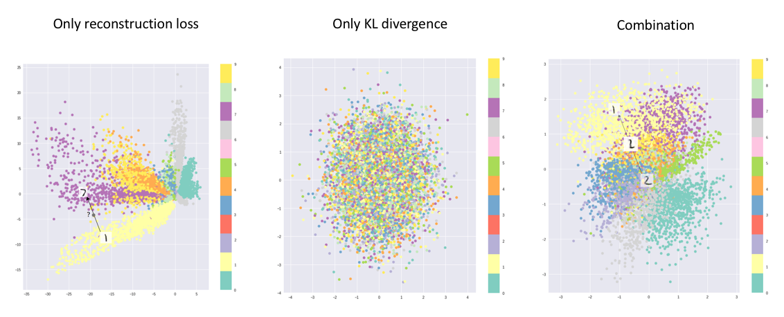
A t-sne visualization of AE's latent space (left-most) v.s. VAE (right-most)
Variational Autoencoders
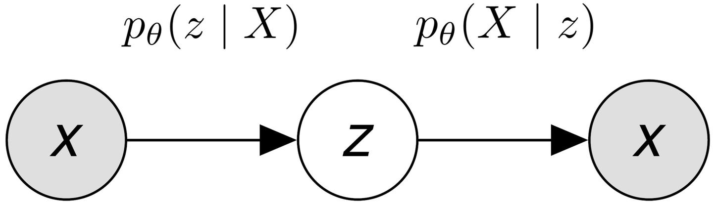
The Probabilistic Model
AEs cannot be sampled from, so we need a probabilistic model. Suppose we can fit \(p(x)\) into a probabilistic space, where:
- \(z\) is the latent space.
- Encoder is \(p_{\theta} (z | X)\)
- Decoder is \(p_{\theta} (X|z)\).
Hypothesis
To facilitate calculations and make the latent space smooth and compact, we make the following assumptions.
We suppose the following distributions are gaussian:
- \(p(z)\): The marginal distribution of latent space is \(\mathcal{N}(0, 1)\).
- \(p_{\theta}(X|z)\): The Decoded real-world distribution given z is some \(\mathcal{N}\)
We can prove that:
- \(p_{\theta} (z | X)\): The
Encoded latent distribution given X is some \(\mathcal{N}\).
This is verified numerically by me, but can be proved.
Network Structure
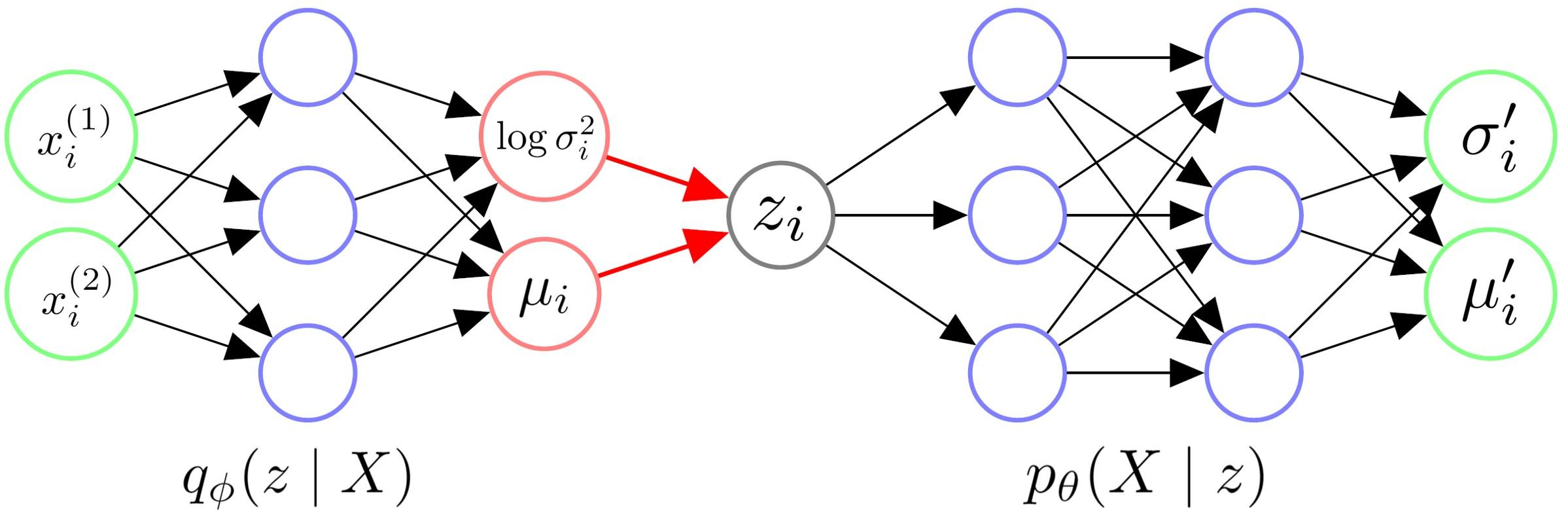
Remark:
- Sometimes, we think \(\mu_{i}'\) is the generated image and ignore \(\sigma_{i}'\). When training, \(\sigma_{i}'\) is a fixed hyperparameter, usually takes \(\frac{1}{2}\). This value will be explained later.
- Since sampling \(z_{i}\) makes backprop unavailable, we generate a \(N(0, 1)\) first and shift/scale it, so that the gradients can backprop to \(\sigma_{i}\) and \(\mu_{i}\) successfully. This is known as "reparameterize trick".
- Since we want \(\sigma_{i}\) to be positive, so we let the model output \(\log {\sigma_{i}^2}\).
Deriving Our Objective
First, we focus on the decoder. We want the model decoded marginal distribution \(p_\theta (x)\) as close to real distribution \(p(x)\) as possible. This is to ensure the normal function of "generating images, xxx..."
Our objective is to make \(p_{\theta}(x)\) close to \(p(x)\). \[ p_\theta(x) = \int p(z) p_\theta(x|z)dz = \mathbb{E}_{z}[p_{\theta}(x|z)] \] Where: 1. \(p_\theta(z)\) is the latent distribution 2. \(p_\theta(x|z)\) is the mapping function
Remark: Since the decoded x is gaussian, such \(p(x_{i} | z_{i})\) is calculable. We can first forward the network to get \(\mu\) and \(\sigma\), then substitute the multivariate gaussian to get the probability expression.
Optimizing \(p_\theta(x)\) Directly
On a discrete case, where \(x_{i} \in \{X\}\) is a dataset, we can minimize the cross-entropy loss between \(p_{\theta} (x)\) and \(p(x)\). This is equivilant to minimizing negative log likelihood (NLL): \[ \theta^* = \arg \min_{\theta} -\sum_{i=1}^n \log p_{\theta}(x_i) \] Where \(p_{\theta}\) can be estimated using monte carlo with random sample \(z_{i}\): \[ p_{\theta}(x_{i}) \approx \frac{1}{m}\sum_{j=1}^m p_{\theta}(x_{i} | z_{i}) \]
We have a problem here: sampling \(z \sim N(0, 1)\) is expensive and not focus. Most \(p_{\theta}(x_i | z_{i})\) are very small since such z are not corresponding to x. Only very few z that are encoded by x can be decoded.
Importance Sampling on \(z_{i}\)
Since sampling \(z_i \sim N(0, 1)\) is bad, we can do importance sampling. We want to use those \(z_{i}\)'s which are most relevant to \(x\). This is exactly what the encoder gives us.
Hence, we give the following target to maximize:
\[ \begin{aligned} -\log p_{\theta}(x_{i}) &= - \log \int p_{\theta}(x_{i} | z) p(z) \frac{q_{\phi}(z|x_{i})}{q_{\phi}(z|x_{i})} dz \\ &= -\log \mathbb{E}_{q_{\phi}(z|x_{i})} \frac{ {p_{\theta}(x_{i}|z)p(z)} }{q_{\phi}(z|x_{i})} \end{aligned} \]
We wish to maximize NLL, i.e. \(-\log p_{\theta}(x_{i})\) Or equivilantly, minimize \(\log p_{\theta}(x_{i})\)
However, using importance sampling to solve the previous, low-efficient optimization process is still not enough. We will prove that the above optimization target is still numerically unstable, and why the following ELBO is better in discussion part
Solution: ELBO
The loss term actually looks quite similar to KL Divergence. However, KL Divergence requires the log to be inside the integral.
Hence, we use jenson's inequality to "move" the log inside: \[ \log p_{\theta}(x) \geq \mathbb{E}_{q_{\phi}(z|x)} \left[ \log \frac{p_{\theta}(x | z) p(z)}{q_{\phi}(z|x)} \right] \] Thus we get the Evidence Lower Bound (ELBO) as follows: \[ \log p_{\theta}(x) \geq \mathbb{E}_{q_{\phi}(z|x)} [\log p_{\theta}(x|z)] - D_{KL}(q_{\phi}(z|x) || p(z)) \]
- The first part is reconstruction term, indicating how far is \(p_{\theta}(x)\) from \(p(x)\).
- The second part is the regularization term, requiring the \(q_\phi(z|x)\) as big as possible (specifically, the loss requires it to be similar to \(p(z)\)), so that the latent space can be more continuous and smooth.
How to Calculate Loss Now
Part 1: The "Reconstruction" Term
\(\mathbb{E}_{q_{\phi}(z|x)} [\log p_{\theta}(x|z)]\) is calculated by: First, generate some samples \(z_{i}\) by encoder; Second, decode them all and calculate their mean; Finally, the loss is the L2 distance between this decoded mean image and X.
Mathematically, this is: \[ \mathbb{E}_{q_{\phi}}[\log p_{\theta}(X | z)] \approx \frac{1}{m}\sum_{i=1}^m \log p_{\theta} (X | z_{i}) \] where \(z_{i} \sim q_{\phi}(z | x_{i})\). We can expand this loss as: \[ \begin{aligned} \log p_{\theta} (X \mid z_i) &= \log \frac{\exp\left(-\frac{1}{2} (X - \mu')^{\top} \Sigma'^{-1} (X - \mu') \right)}{\sqrt{(2\pi)^k |\Sigma'|}} \\ &= -\frac{1}{2} (X - \mu')^{\top} \Sigma'^{-1} (X - \mu') - \log \sqrt{(2\pi)^k |\Sigma'|} \\ &= -\frac{1}{2} \sum_{k=1}^{K} \frac{(X^{(k)} - \mu'^{(k)})^2}{\sigma'^{(k)2}} - \log \sqrt{(2\pi)^K \prod_{k=1}^{K} \sigma'^{(k)2}}. \end{aligned} \] Where \(\sigma', \mu'\) needs to be inferenced after sampling a \(z_i\), using decoder.
Part 2: The KL Divergence Term
We start from calculating 1d case first.
\[ \begin{aligned} D_{KL}&(\mathcal{N}(\mu, \sigma^2) \| \mathcal{N}(0, 1)) \\ &= \int_{z} \frac{1}{\sqrt{2\pi\sigma^2}} \exp\left( -\frac{(z - \mu)^2}{2\sigma^2} \right) \log \frac{\frac{1}{\sqrt{2\pi\sigma^2}} \exp\left( -\frac{(z - \mu)^2}{2\sigma^2} \right)}{\frac{1}{\sqrt{2\pi}} \exp\left( -\frac{z^2}{2} \right)} dz \\ &= \int_{z} \left( -\frac{(z - \mu)^2}{2\sigma^2} + \frac{z^2}{2} - \log \sigma \right) \mathcal{N}(\mu, \sigma^2) dz \\ &= - \int_{z} \frac{(z - \mu)^2}{2\sigma^2} \mathcal{N}(\mu, \sigma^2) dz + \int_{z} \frac{z^2}{2} \mathcal{N}(\mu, \sigma^2) dz - \int_{z} \log \sigma \mathcal{N}(\mu, \sigma^2) dz \\ &= - \frac{\mathbb{E}[(z - \mu)^2]}{2\sigma^2} + \frac{\mathbb{E}[z^2]}{2} - \log \sigma \\ &= \frac{1}{2}(-1 + \sigma^2 + \mu^2 - \log \sigma^2) \end{aligned} \]
For a i.i.d multivariable case, the loss is:
\[ D_{KL} \left( q_{\phi}(z \mid X), p(z) \right) = \sum_{j=1}^{d} \frac{1}{2} \left( -1 + \sigma^{(j)^2} + \mu^{(j)^2} - \log \sigma^{(j)^2} \right). \]
The Loss Function, Merged
Given a size \(n\) minibatch, the final loss is: (suppose for each \(\mathbb{E} q_{\phi}\), we sample \(m\) times.)
\[ \begin{aligned} \mathcal{L} &= -\frac{1}{n} \sum_{i=1}^{n} \ell(p_{\theta}, q_{\phi}) \\ &= \frac{1}{n} \sum_{i=1}^{n} D_{KL} \left( q_{\phi}, p \right) - \frac{1}{n} \sum_{i=1}^{n} \mathbb{E}_{q_{\phi}} \left[ \log p_{\theta} (x_i \mid z) \right] \\ &= \frac{1}{n} \sum_{i=1}^{n} D_{KL} \left( q_{\phi}, p \right) - \frac{1}{nm} \sum_{i=1}^{n} \sum_{j=1}^{m} \log p_{\theta} (x_i \mid z_j). \\ \end{aligned} \]
In practical, we find that \(m = 1\) is fine as well. Hence the loss can be even simplified to:
\[ \begin{aligned} \mathcal{L} &= \frac{1}{n} \sum_{i=1}^{n} D_{KL} \left( q_{\phi}, p \right) - \frac{1}{n} \sum_{i=1}^{n} \log p_{\theta} (x_i \mid z_i) \\ &= \frac{1}{n} \sum_{i=1}^{n} \sum_{j=1}^{d} \frac{1}{2} \left( -1 + \sigma_i^{(j)2} + \mu_i^{(j)2} - \log \sigma_i^{(j)2} \right) \\ &\quad - \frac{1}{n} \sum_{i=1}^{n} \left( \frac{1}{2} \sum_{k=1}^{K} \frac{(x_i^{(k)} - \mu_i'^{(k)})^2}{\sigma_i'^{(k)2}} - \log \sqrt{(2\pi)^K \prod_{k=1}^{K} \sigma_i'^{(k)}} \right). \end{aligned} \]
We can let \(\sigma'^{(k)}\) (a hyperparameter, mentioned before) as \(\frac{1}{2}\), hence the loss can be simpliflied to:
\[ \begin{aligned} \mathcal{L}_{\text{VAE}} = &\frac{1}{n} \sum_{i=1}^{n} \sum_{j=1}^{d} \frac{1}{2} \left( -1 + \sigma_i^{(j)2} + \mu_i^{(j)2} - \log \sigma_i^{(j)2} \right) \\ &+ \frac{1}{n} \sum_{i=1}^{n} \left\| x_i - \mu'_i \right\|^2. \end{aligned} \]
This is the final VAE Loss, i.e. adding
- a recon loss (L2 loss) on ground truth image and recon image,
- and a regularization term
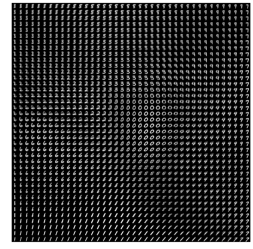
Remark: If you want to use F.mse_loss, make sure to
multiply the loss by \(H*W\), since
torch mse loss divide it! This is important becuase it will affect the
strength of recon loss. If recon loss is very small, the image will be
evenly scattered in the latent space, instead of structured scattered.
(Middle figure below)
VAE, Summarized
Intuition
- The encoder maps \(x\) to \(z\).
- But we need to be able to sample from \(p(z)\).
- So we need encoder to learn \(p(z|x)\) (probabilistic) instead of \(f(x)=z\) (deterministic)
- But how to get \(p(z|x)\) (encoder)?
- Partial solution: Bayes rule, calculate \(\frac{p(x|z)p(z)}{p(x)}\)
- Problem: What is \(p(x)\)?
- Solution: learn \(q(z|x)\) directly, and make it close to \(p(z|x)\)
- How to regularize? Requre \(q(z|x)\) to be close to \(p(z)\) as well!
Loss Term
- Optimize ELBO \[ \max \log p(x) \ge \mathbb{E}_{q(z|x)} \log p(x|z) - DL( q(z|x) || p(z) ) \]
maximize decoder \(p(x|z)\) while regularize \(q(z|x)\) to be close to \(p(z)\) where KL Div here are closed form if we use gaussians for p and q
Key feature
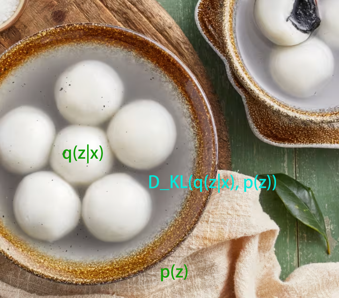
VAE is "denser" and interpolations matters!!
Each "Tang yuan" has its space, but you want to maximize its space! (so that their won't be so much gaps between "Tang Yuan" and the bowl.) (This is achieved by KL Divergence loss term.)
Also, make them seperate from each other. (This is achieved by reconstruction loss term.)
Discussion
Entropy Intuition
Recommended Reading: Understanding Entropy
Intuition 1: how random is X
Intuition 2: how large is the log probability in expectation under
itself
\[ \mathcal{H(p)} = E_{x \sim p(x)} [-\log p(x)] = \int_{\mathcal{X}} [-p(x) \log p(x)]dx = -\sum_{x \in \mathcal{X}}[p(x)\log p(x)] \]
Intuitive 3: What is the least encoding length of this message (suppose we encode more-frequent messages with less bits, just like Huffman Coding)
As a result, we always want to:
- Maximize information, i.e. maximize \(-\log p_{\theta}(x)\)
- Minimize entropy, i.e. minimize \(-E_{x \sim p(x)} \log p(x)\)
Cross Entropy, KL Divergence Intuition
KL Divergence is defined as the gap of entropy, i.e. \(D_{KL}(p \| q) = H(p, q) - H(p)\), where:
\[ H(p, q) = \mathbb{E}_{x \sim p(x)} [-\log q(x)] = \int_{\mathcal{X}} [-p(x)\log q(x)] dx = -\sum_{x \in \mathcal{X}} [p(x) \log q(x)] \]
I.f.f "model distribution (q)" is equal to "realistic distribution (p)", cross entropy is equal to entropy, i.e. \(H(p, p) = H(p)\)
The full, expanded definition is:
\[ D_{\mathrm{KL}}(p\|q) \;=\; \sum_{x\in\mathcal X} p(x)\,\log\!\biggl(\frac{p(x)}{q(x)}\biggr) \;=\; \mathbb{E}_{x\sim p}\Bigl[\log p(x) - \log q(x)\Bigr]. \]
As a result, we always want to:
- Minimize KL Divergence, i.e. minimize \(H(p, q) - H(p)\)
Remark: We can prove that KL Divergence is always positive. Proof: use jenson's inequality on \(-D_{KL}\), which only leaves \(\log q(x)\), which is always negative. Hence \(D_{KL}\) is always positive.
Remark: We can prove that minimizing KL is equivilant to minimizing NLL. Proof:
\[ \begin{aligned} KL(p \| p_\theta) &= \mathbb{E}_p [\log \frac{p(x)}{p_\theta(x)}] \\ &= \underbrace{\mathbb{E}_{p}\!\bigl[-\log p_\theta(x)\bigr]}_{=\mathcal{L}_{\text{NLL}}(\theta)} - \underbrace{\mathbb{E}_{p}\!\bigl[-\log p(x)\bigr]}_{=H\!\left(p\right)} \end{aligned} \]
Another Perspective on ELBO
We want to know: What are we "dropping" on ELBO, i.e.
\[ \text{original} - \text{ELBO bound} := \text{dropped terms} \ge 0 \]
The derivation is:
\[ \begin{aligned} \log p_{\theta}(X) &= \int_{z} q_{\phi}(z \mid X) \log p_{\theta}(X) dz \\ &= \int_{z} q_{\phi}(z \mid X) \log \frac{p_{\theta}(X, z)}{p_{\theta}(z \mid X)} dz \\ &= \int_{z} q_{\phi}(z \mid X) \log \left( \frac{p_{\theta}(X, z)}{q_{\phi}(z \mid X)} \cdot \frac{q_{\phi}(z \mid X)}{p_{\theta}(z \mid X)} \right) dz \\ &= \int_{z} q_{\phi}(z \mid X) \log \frac{p_{\theta}(X, z)}{q_{\phi}(z \mid X)} dz \\ & + \quad \int_{z} q_{\phi}(z \mid X) \log \frac{q_{\phi}(z \mid X)}{p_{\theta}(z \mid X)} dz \\ &= \ell(p_{\theta}, q_{\phi}) + D_{KL}(q_{\phi} \parallel p_{\theta}) \\ &\geq \ell(p_{\theta}, q_{\phi}) \end{aligned} \]
We can find that \(\ell (p_{\theta}, q_{\phi})\) is exactly the ELBO bound! Prove is as follows:
\[ \begin{aligned} \ell (p_{\theta}, q_{\phi}) &= \int_{z} q_{\phi}(z \mid X) \log \frac{p_{\theta}(X, z)}{q_{\phi}(z \mid X)} dz \\ &= \int_{z} q_{\phi}(z \mid X) \log \frac{p_{\theta}(X \mid z)p(z)}{q_{\phi}(z \mid X)} dz \\ &= \int_{z} q_{\phi}(z \mid X) \log \frac{p(z)}{q_{\phi}(z \mid X)} dz + \int_{z} q_{\phi}(z \mid X) \log p_{\theta}(X \mid z) dz \\ &= - D_{KL} (q_{\phi}, p) + \mathbb{E}_{q_{\phi}} [\log p_{\theta}(X \mid z)]. \\ &= \text{ELBO_bound} \end{aligned} \]
So, it is easy to find that
\[ \log p_{\theta}(x) - \text{ELBO_bound} = D_{KL}(q_{\phi} \| p_{\theta}) \]
This means that we are actually dropping a intractable KL term from our loss! (since it requires \(p_\theta\))
Why ELBO is better than optimizing NLL directly?
Here we restate the above problem: Suppose we are optimizing \(-\log \mathbb{E}_{q_\phi (z | x_i)} w(z)\), where \(w(z) = p_\theta (x_i | z) p(z) / q_\phi (z | x_i)\). Or, by the aforementioned re-parameterization trick, this is: \(-\log \mathbb{E}_{\epsilon \sim N(0, I)} w(\epsilon)\).
Suppose we want to know the optimization target's gradient to our parameters in encoder, i.e. \(\theta\). Here is its value:
\[ \begin{aligned} \nabla_\theta & (-\log \mathbb{E}_\epsilon w(\epsilon)) \\ &= -\frac{1}{\mathbb{E}_\epsilon w(\epsilon)} \cdot \mathbb{E}_\epsilon \nabla_\theta (w(\epsilon)) \\ &= -\frac{1}{\mathbb{E}_\epsilon w(\epsilon)} \cdot \mathbb{E}_\epsilon [\frac{p(z)}{q_\phi (z | x_i)} \cdot \nabla_\theta p_\theta(x_i | z)] \\ &= -\frac{1}{\mathbb{E}_\epsilon w(\epsilon)} \cdot \mathbb{E}_\epsilon [\frac{p(z) p_\theta(x_i | z)}{q_\phi (z | x_i)} \cdot \frac{\nabla_\theta p_\theta(x_i | z)}{p_\theta(x_i | z)}] \\ &= -\frac{1}{\mathbb{E}_\epsilon w(\epsilon)} \cdot \mathbb{E}_\epsilon [w(\epsilon) \cdot \nabla_\theta \log p_\theta(x_i | z)] \\ &= -\mathbb{E}_\epsilon [\frac{w(\epsilon)}{\mathbb{E}_\epsilon w(\epsilon)} \cdot \nabla_\theta \log p_\theta(x_i | z)] \end{aligned} \]
Here we found the term \(\frac{w(\epsilon)}{\mathbb{E}_\epsilon w(\epsilon)}\) annoying, since it requires an additional sampling on each datapoint \(x_i\) to calculate this coefficient, increasing the variance and unstability. Also, it is numerically unstable due to the denominator can be close to 0. Let's see how ELBO does better:
ELBO is trying to optimize: \(-\log \mathbb{E}_{\epsilon} w(\epsilon) \approx \mathbb{E} [-\log w(\epsilon)]\) (should be inequality here), lets deriviate its gradient to see why its stabler and don't rely on sampling the inner coefficient:
\[ \begin{aligned} \nabla_\theta & \mathbb{E}_\epsilon [-\log w(\epsilon)] \\ &= \mathbb{E}_\epsilon [\nabla_\theta [-\log w(\epsilon)]] \\ &= \mathbb{E}_\epsilon [\nabla_\theta \log p_\theta(x_i | z)] \end{aligned} \]
Here, the annoying coefficient disappears! And we can directly calculate the loss for each datapoint \(x_i\) with only one sampling process on \(\epsilon\) (or \(z\), equivilantly), instead of sampling on \(\epsilon\) twice. Also, we avoid the can-be-zero denominator in the first case.
Drawbacks on VAE
We usually say that VAE generated images are blurry. Why?
[D]Why are images created by GAN sharper than images by VAE? : r/MachineLearning Answer: Vanilla VAEs with Gaussian posteriors / priors and factorized pixel distributions aren't blurry, they're noisy. People tend to show the mean value of p(x|z) rather than drawing samples from it. Hence the reported blurry samples aren't actually samples from the model, and they don't reveal the extent to which variability is captured by pixel noise. Real samples would typically demonstrate salt and pepper noise due to independent samples from the pixel distributions.
Another view: \(p(x)\), in real world, is not gaussian. They are usually multi-peak, instead of gaussian (single-peak). Hence averaging multi-peaks will result in blurry image.
CVAE: Adding Class Condition
We just need the model to be parameterized by label \(c_{i}\) as well. A simple solution is:
| Term | Previous | Now |
|---|---|---|
| Original Distribution | \(p_{\theta}(x)\) | \(p_{\theta}(x \| c)\) |
| Latent Distribution | \(p(z)\) | \(p(z \| c)\) |
| Encoder | \(p_{\theta}(x \| z)\) | \(p_{\theta}(x \| z, c)\) |
| Decoder | \(q_{\phi}(z \| x)\) | \(q_{\phi}(z \| x, c)\) |
Implementing VAE & CVAE
Reference solution: Machine-Learning-with-Graphs/examples/MLMath/VAE.py
at main · siqim
Very short but effective. ~100 lines of code per method.
Modern VAEs in LDM
Why is VAE still very useful in Latent Diffusion Models, though it generates blurry image?
| Traditional VAE | VAE in LDM | |
|---|---|---|
| Purpose | As a generative model | As an autoencoder |
| Latent | Compressed into a single vector | Compressed into a*b vectors |
| Reconstruction Loss | MSE | MSE + Perceptual loss + Adversarial loss |
| Regularization Term | Complete KL divergence term | Weakened KL divergence term |
| Purpose of Regularization | To enable VAE to function as a generative model | To make the distribution of the latent space smoother and smaller for easier training of the diffusion model |
Excessive compression, the use of only MSE for reconstruction loss, and the complete KL divergence term are the reasons for the blurriness of traditional VAEs. For traditional VAEs, improving the reconstruction loss is essential. In fact, if you replace the reconstruction loss of a traditional VAE with "MSE + Perceptual loss + Adversarial loss," the blurriness of the VAE will also be significantly reduced.
However, modifying the reconstruction loss can only solve the blurriness issue and cannot address the problem of compression-induced information loss. Compressing an 256*256 image into a single-dimensional vector inevitably results in severe information loss, retaining only high-level semantic features while losing detailed texture information.
Given this, the VAE in LDM is responsible only for compressing the image size and not for being a generative model (this task is left to the diffusion model). For example, instead of compressing into a single-dimensional vector, it preserves an a*b dimensional feature map, allowing each point to retain meaningful information. Then, the KL divergence term is weakened (or VQ-VAE uses a VQ term instead), allowing for a smoother latent space. As a result, it is no longer necessary to optimize the reconstruction loss further.
In summary, the VAE in LDM is only responsible for producing clear results (with a minor regularization term), and its generative capability comes from the diffusion model rather than functioning as a traditional VAE.
About SGVB and AEVB
From the original paper, these two terms are:
- SGVB: focus on reparameterization and grad descent
- AEVB: the whole VAE structure, as a auto encoder and bayes inference method.