MeshEdit

Computer Graphics Rasterization

 2025/03/04 

Overview

This project implemements:

Bezier Curves / Surfaces' Evaluation
Halfedge-Based Mesh Traversal & Editing, including:
1. Vertex Normals
2. Edge Flip & Split (with Boundary Handling)*
3. Loop Subdivision (with Boundary Handling)* and case study on its effect

The ones marked with an asterisk (*) are my bonus implementations.

Task 1: 2D Bezier Curve

Algorithm Overview

First, we implement the 2D Bezier Curve.

Here is a short pipeline for De Casteljau's Algorithm, which provides a way to eval Bézier curves at any parameter value $t$. In the simplest view, this is an iterative interpolating function:

Start with $n+1$ control points $P_0, P_1, \cdots, P_n$defining a Bézier curve of degree $n$.
While remaing control points $m > 1$, do the following loop:
1. For a parameter value $t$ (where $0 \le t \le 1$):
  1. Perform $n$ iterations of linear interpolation: $P^{(i+1)}_j = t \cdot P^{(i)}_j + (1-t) \cdot P_{j+1}^{(i)}$
2. The process reduces $m$ points to $m-1$ points
The final point $P^{(n)}_0$ is the point on the Bézier curve at parameter t.

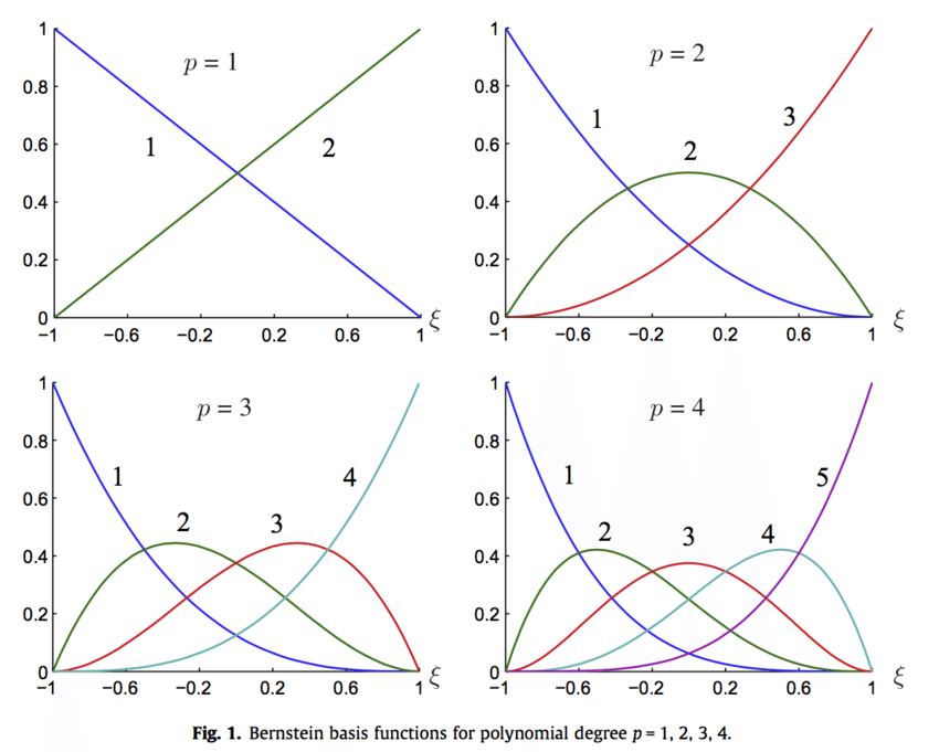
Also, from a high-level understanding, we can treat each control point as a basis. Hence each interpolated point can be expressed as a weighted sum of basis, given as:

\[ B(t) = \sum_{i=0}^{n} B_i^n (t) p_i \\ B_i^n (t) = \binom{n}{i} (1 - t)^{n-i} t^i \] where:

$B(t)$ is the equation of Bézier curves
$B_i^n (t) $ is Bernstein Basis function
$ p_i $ is each control point
$ t $ is the interpolation parameter

Bernstein basis functions for polynomial degree p = 1, 2, 3, 4. | Download Scientific Diagram

Result Gallery

The interpolation process of Bezier Curve

Different interpolation parameter ($t$), visualized

One different control point can have effect on the whole curve (Non-locality of Bezier Curves)

Task 2: 3D Bezier Surface

Algorithm Overview

De Casteljau's algorithm extends to Bézier surfaces by applying the algorithm twice: once in the first direction (e.g., $u$) and then in the other (e.g., $v$). Suppose we have the control points defined as: $p_{i,j}$ for $i = 0, \dots, n$ and $j = 0, \dots, m$. The interpolation steps are as follows:

Apply de Casteljau in One Direction (e.g., $u$)
- For a fixed $v$, treat each row of control points $\{ p_{i,j} \}_{i}^{n}$ as a Bézier curve in $u$.
- Use de Casteljau’s algorithm to compute intermediate points recursively until reaching a single point per row.
- This is: from $n*n$ points to $n*1$ points
Apply de Casteljau in the Second Direction (e.g., $v$)
- Use de Casteljau’s algorithm again along this new curve to obtain the final point on the surface for given parameters $(u,v)$.
- This is: from $n*1$ points to $1*1$ point.
Repeat for Different u, v Values: This process is repeated for different values of $u$ and $v$ to generate the full Bézier surface.

This recursive approach allows Bézier surfaces to be efficiently evaluated and subdivided, just like Bézier curves.

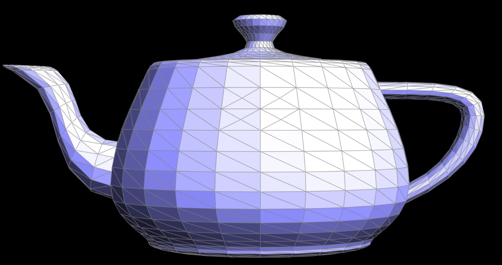
Result Gallery

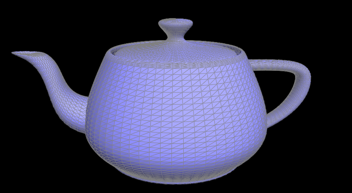
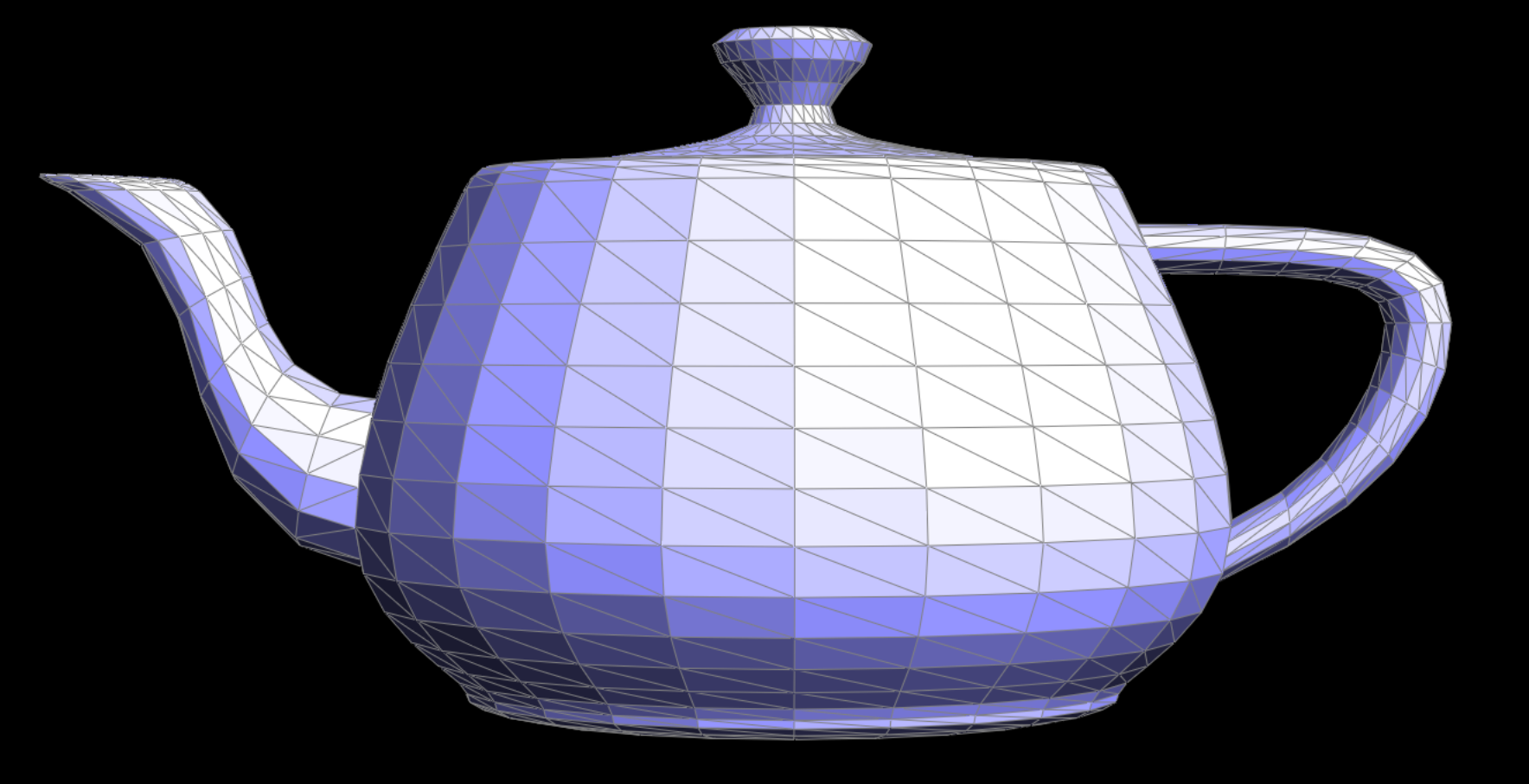
A rendered teapot, defined by Bezier surfaces.

Task 3: Vertex Normals

Algorithm Overview

Using vertex normals, we can enable smooth shading by interpolating vertex colors in triangles.

The algorithm to iterate through all non-boundary faces neighbouring v is given as follows:

Let h be any halfedge starting from v
Let h_init = h
while (h != h_init):
1. Calculate something using h here...
2. h = h->twin()->next()

Hence, in each loop, we collect h->face()->normal() and do average to get vertex normals. Do remember to omit boundary edges since they are consisted of mulltiple edges (>3), which do not have normals.

Result Gallery

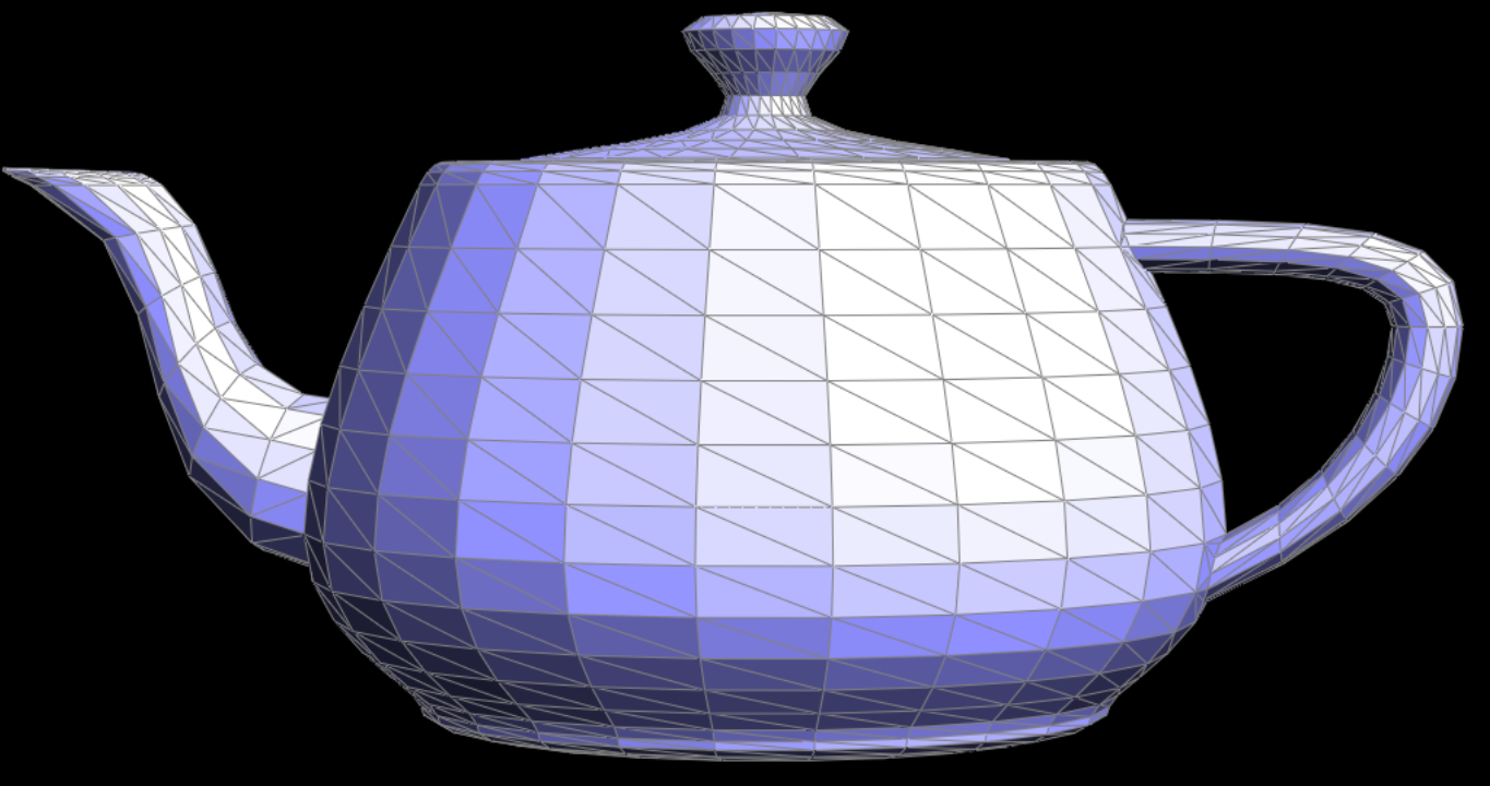
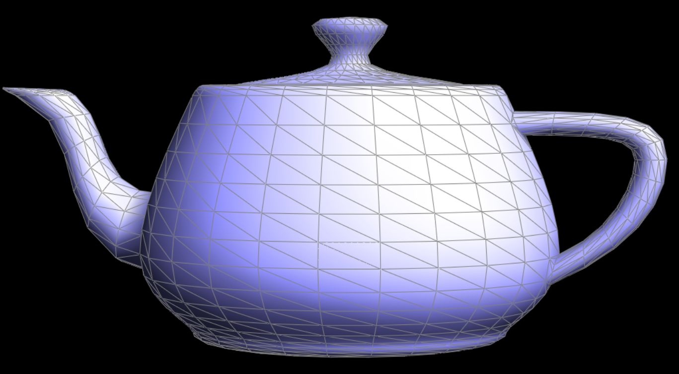
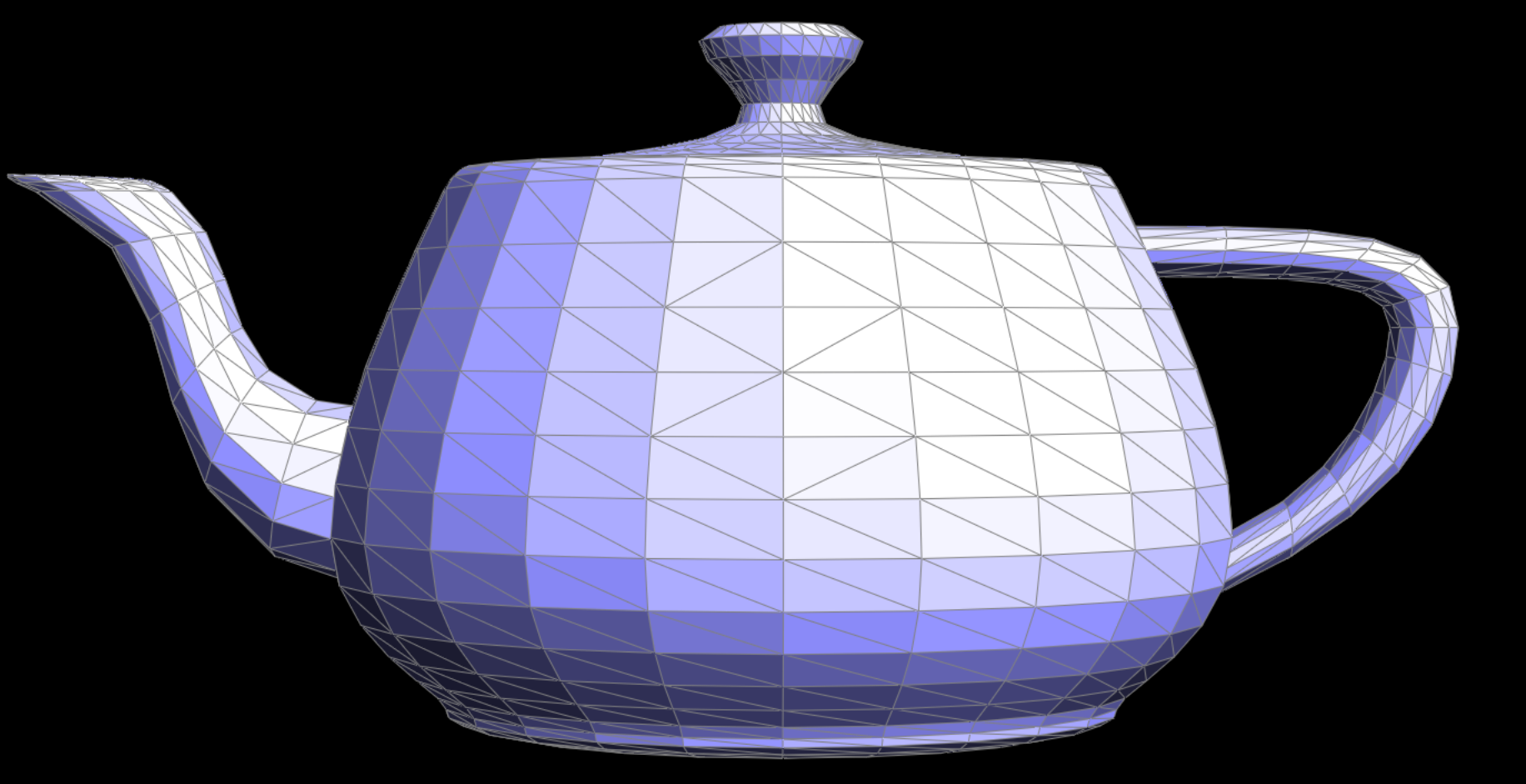
A rendered teapot, using vertex normals to interpolate colors (Right, Smooth Shading).

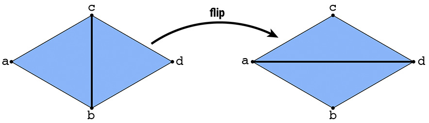
Part 4: Flip Edge

For your reference, here is a short notation clarification for variables afterwards.

Variables starting with f are faces
Variables starting with e are edges
Variables starting with h are halfedges
Variables starting with v are vertices

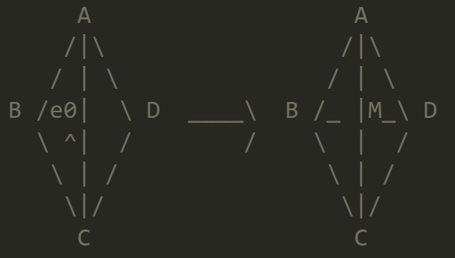
Algorithm Overview

Actually, in a edge flip, we do not necessarily need to create new elements and delete old elements. We can think of it as an internal rotation, where fABC, fCBD and eBC are kind of "rotated" into fCAD, fABD and eAD. We just need to update the struct members.

Diagram that details an Edge flip algorithm.

First, to ensure consistency, we collect old edges/vertices/faces. (So that each old iterator points to correct edges, and we don't need to worry being modified in the process.)
Second, the following terms are updated:
1. Halfedges: hDA, hAB, hBD (in face ABD); hAD, hDC, hCA (in face ADC)
2. Vertices: vA, vB, vC, vD.
3. Faces: fABC, fCBD
Return e0

Result Gallery

A rendered teapot, with some edges before & after flipped.

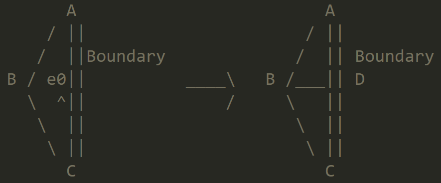
Part 5: Split Edge

Boundary Case

Here is the case when we are splitting boundary edges. Pay special attention that we don't split boundary faces!

First, to ensure consistency, we collect old edges/vertices/faces. (So that each old iterator points to correct edges, and we don't need to worry being modified in the process.)
Second, the following terms are updated:
1. Create: hDA, hDA, hCD, hDC, hBD, hDB // eAD, eBD, eCD // fABD, fBCD // vD
2. Update: hAB, hBC // vB, vC
3. Eliminate: hAC, hCA // eAC // fABC
Return vD

Non-Boundary Case

Here is the case when we are splitting non-boundary edges.

First, to ensure consistency, we collect old edges/vertices/faces. (So that each old iterator points to correct edges, and we don't need to worry being modified in the process.)
Second, the following terms are updated:
1. Create: eAM, eMC, eMD, eBM // hAM, hMA, hBM, hMB, hCM, hMC, hDM, hMD // vM // fABM, fAMD, fMCD, fBMC
2. Update: eAB, eBC, eCD, eDA // hAB, hBC, hCD, hDA // vA, vB, vC, vD
3. Eliminate: eAC // hAC, hCA // fABC, fADC
Return vM

Result Gallery


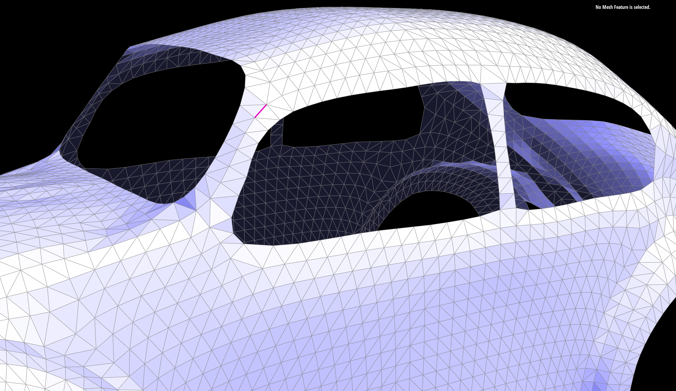
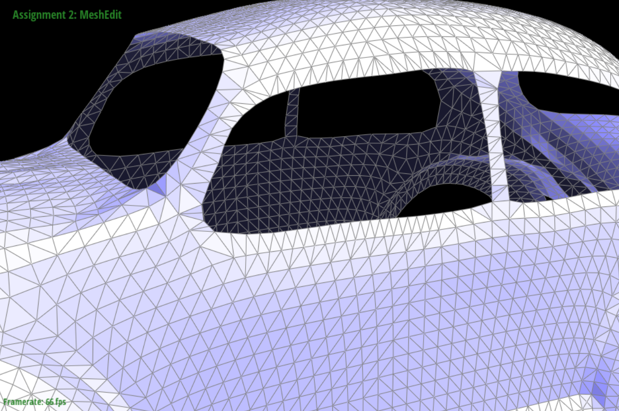
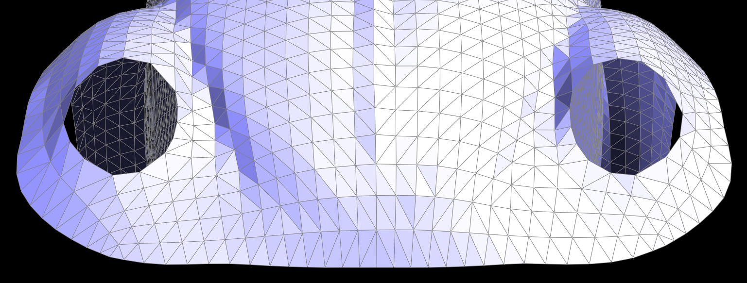
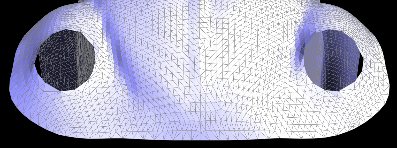
A teapot	A beetle

A teapot, with edges splitted	A beetle, with boundaries splitted

A teapot, with edges splitted and flipped	A beetle, with boundaries splitted and flipped

Task 6: Loop Subdivision

Algorithm Overview

Compute new positions for all the vertices in the input mesh, and store them in Vertex::newPosition.
1. For boundary vertices, we have:
  vpos = (3/4) * orig_position + (1/8) * (neighbor1 + neighbor2)
2. For other vertices, we have:
  vpos = (1 - n * u) * orig_position + u * orig_neighbor_position_sum
Compute the updated vertex positions associated with edges, and store it in Edge::newPosition.
1. For boundary edges, we have epos = 3/8 * (A + B) + 1/8 * (C + D)
2. For other edges, we have epos = (3.0 / 8.0) * (A + B) + (1.0 / 8.0) * (C + D)
Cache all the old edges in std::vector<EdgeIter> originalEdges
For each edge in originalEdges:
1. Read its epos
2. Split edge and get the returned vertex vNew
3. Let vNew's position be epos
4. Iter through all edges starting from vNew:
  1. If this edge connects old mesh points, mark e->isNew = false
  2. Else, mark e->isNew = true
For each edge in mesh.edges:
1. If eIter->isNew and isBoundary() = false, then flip this edge.
Copy the new vertex positions into final Vertex::position.

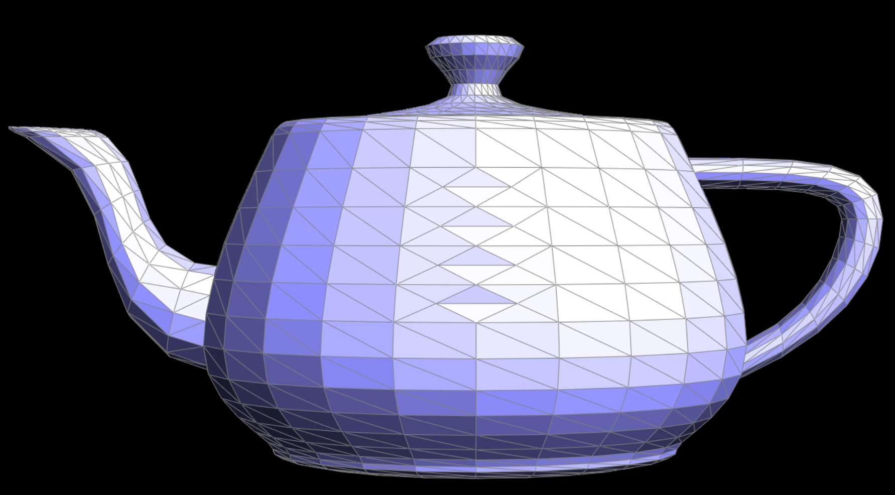
Result Gallery

w/o Loop Subdivision
Loop Subdivision w/o Edge Handling
Loop Subdivision w/ Edge Handling

Overall performance of loop subdivision. As the images show, the edges are "smoothed". With correct edge handling in the loop subdivision algorithm, they can become even "smoother".

	Before Loop Subdivision	After Loop Subdivision
w/o Pre- Splitting
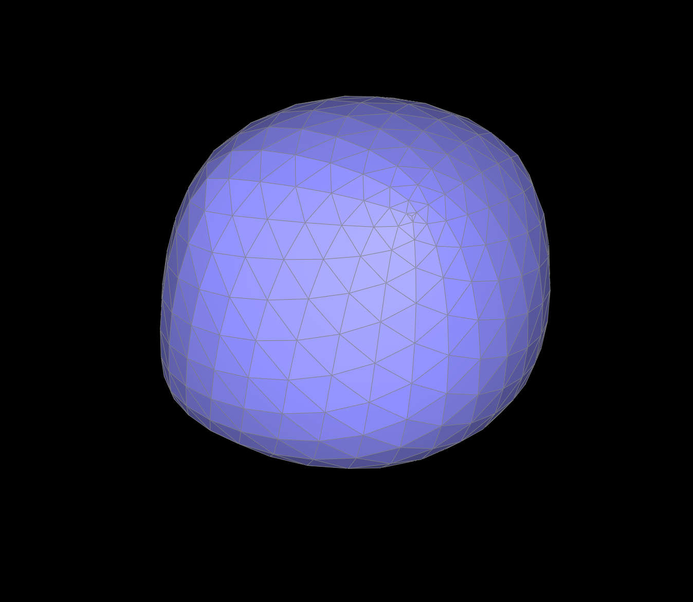
w/ Pre- Splitting

Comparision of w/ Pre-splitting and w/o Pre-Splitting.

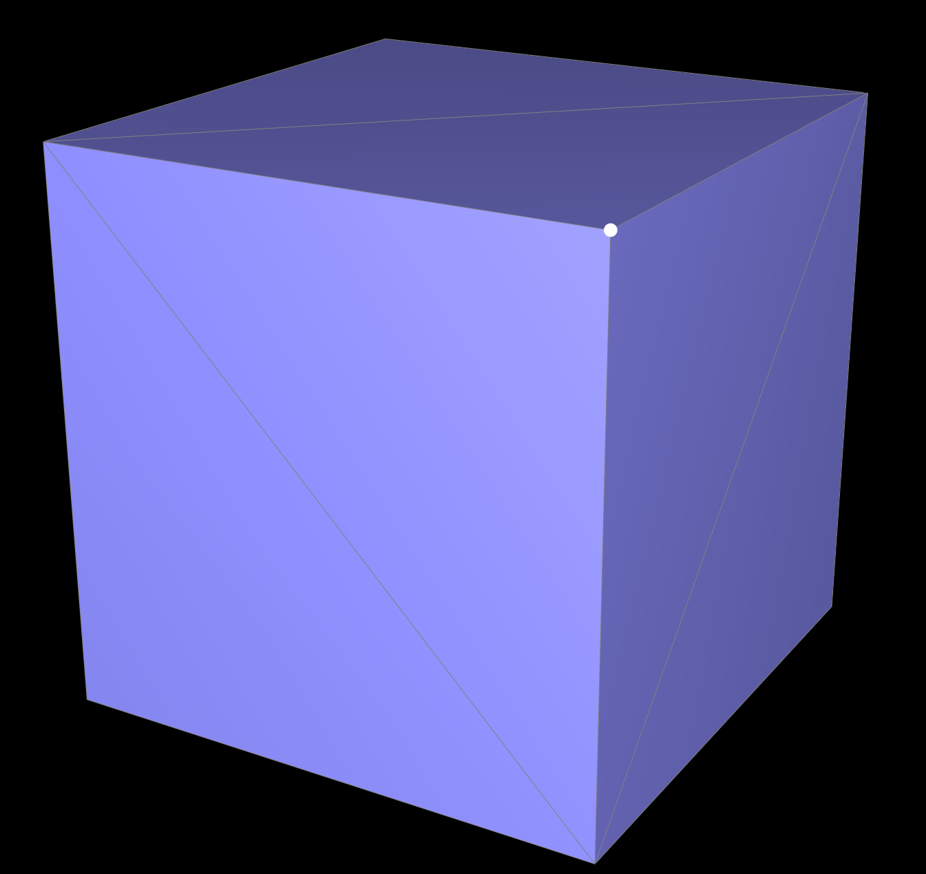
Sometimes, the sharp corners are "smoothed" too much. To reduce this effect, we can manually add some supporting edges near the being-preserved corner. This is effective because Loop Subdivision calculates a local average. Instead of using a vertex on another corner (in the cube) to average, Pre-Splitting allows Loop Subdivision to use a nearer vertex to do average, which preserves the shape of the corner.

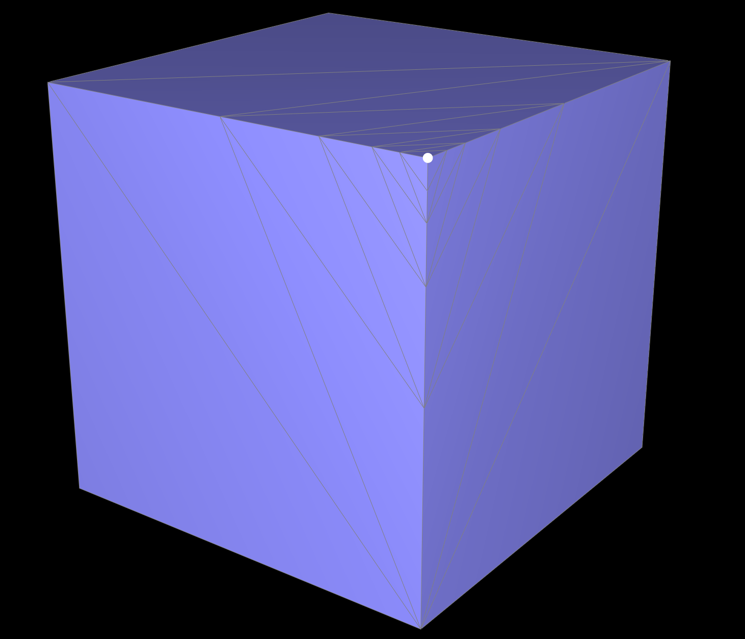
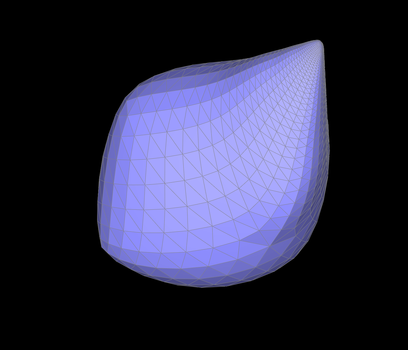
	Before Loop Subdivision	After Loop Subdivision
w/o Pre- Splitting
w/ Pre- Splitting

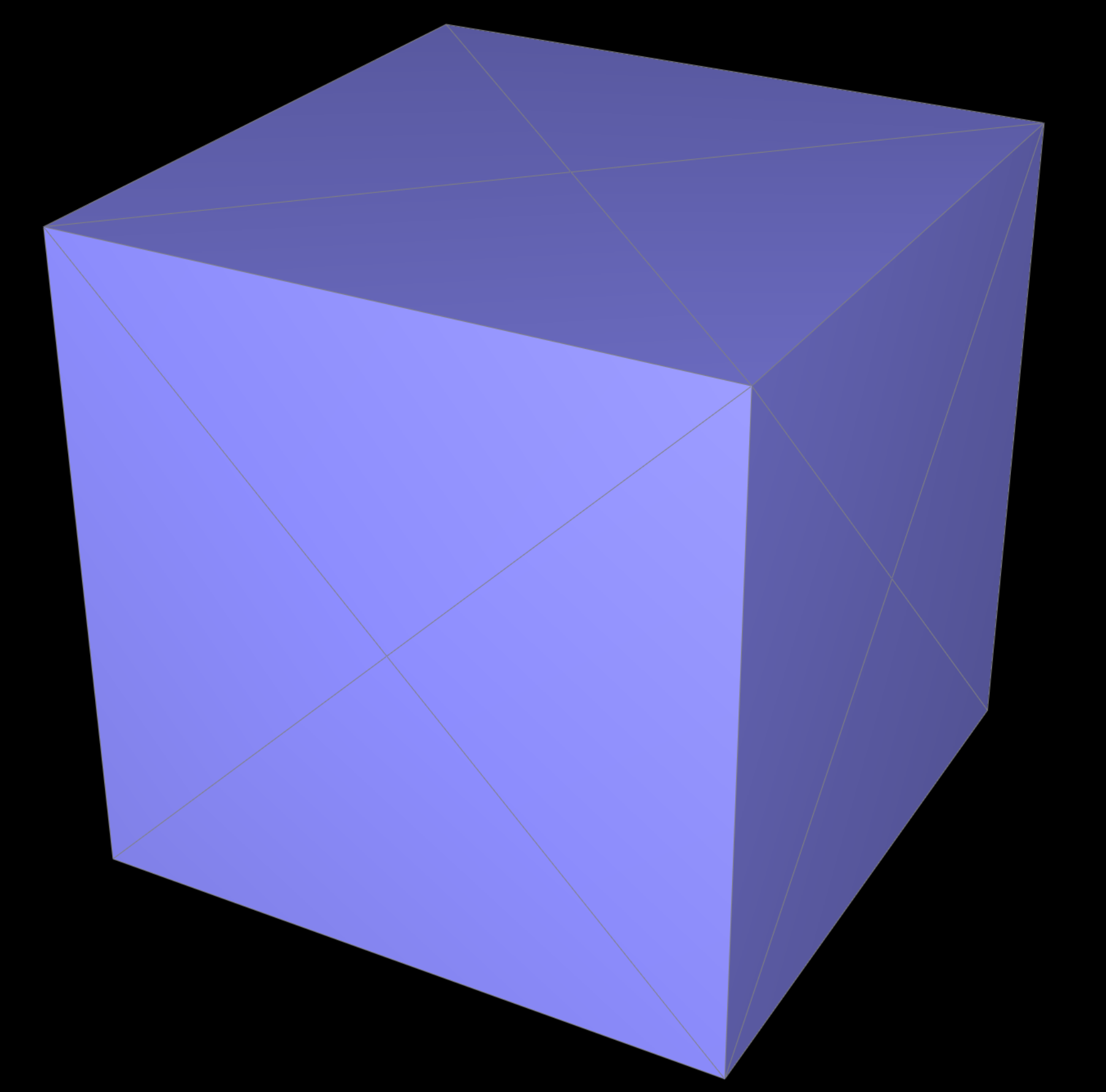
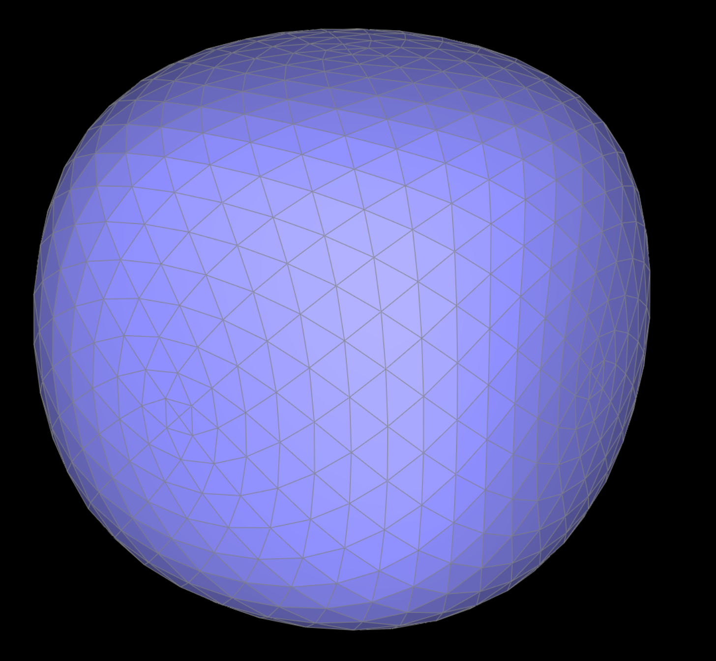
Comparision of w/ Pre-splitting and w/o Pre-Splitting.

Sometimes, the cube becomes asymmetric after division. This is because that the original edges are not splitted symmetricly, hence when Loop Subdivision is finding near points to calculate average, it will look up differently for different corners. However, there is a solution. We manually added more splitted and flipped edges, so that the cube looks like a "X" from each face. Hence all corners are in symmetric states, and the Loop Subdivision will carry out symmetrically as well!

Author：SimonXie2004

Link：https://simonxie2004.github.io/2025/03/04/MeshEdit/

Publish date：March 4th 2025, 3:26:27 am

Update date：April 8th 2025, 11:59:30 pm

License：CC-4.0

Next Post

Re-Inventing VAE on a Retrospective Perspective
Previous Post

Mathematical Derivation of EWA Filtering