
Introduction & Intuition
In texture anisotropic filtering, we have one basic problem: antialiasing. If the projection distortion is big, pixels at further area appear aliased. For example, take a look at this picture:
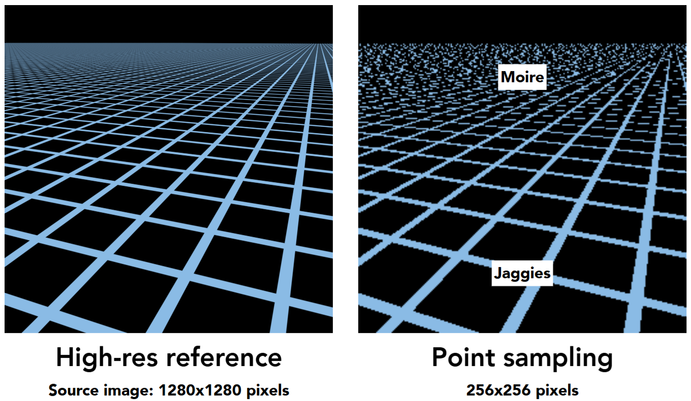
The underlying reason is: different screen-space pixels span different area in texture space.
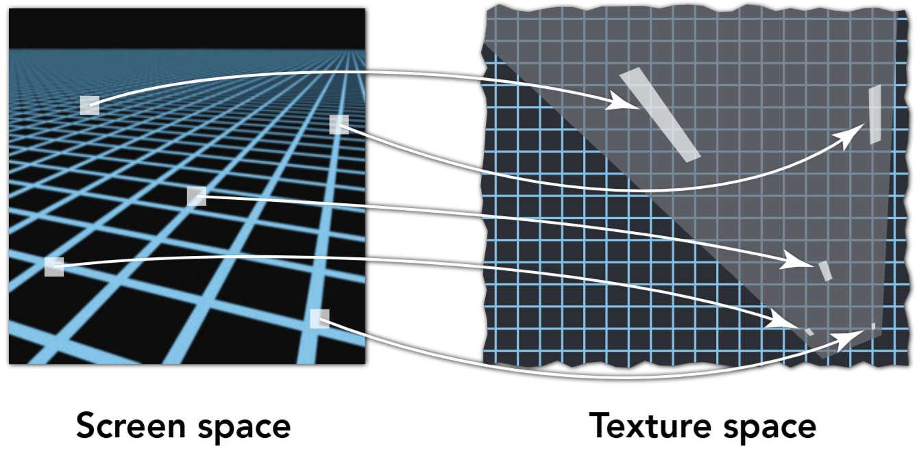
So, we want to know how a pixel in screen space is projected to texture space. This involves two main parts:
- If the pixel is projected to texture space, which area will it span?
- Given the area that a screen pixel span in texture space, how should we average their color?
This is where ewa filtering comes in.
Mathematical Induction
Projecting Pixels
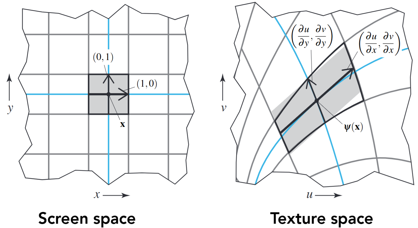
First, we need to know how a screen pixel is projected to texture space. We mainly focus on unit vectors: How are \(dx\) and \(dy\) projected?
The answer is quite simple! You just need to calculate the
barycentric coordinates to determine the
relative position of the points to the triangle
vertices. Then, you may use the barycentric coordinates to
weighted average your vertex uvs. The
pseudocode is:
1 | def project_screen_point_to_uv_space( |
As long as we can project points, we can project vectors!
This is how we calculate \((\frac{du}{dx}, \frac{dv}{dx}), (\frac{du}{dy}, \frac{dv}{dy})\).
Understanding Jacobians (As Linear Transforms)
The above process can be written in a simple mathematical formula, i.e. \[ J = \frac{\partial(u, v)}{\partial(x, y)} = \begin{bmatrix} \frac{du}{dx} & \frac{du}{dy} \\ \frac{dv}{dx} & \frac{dv}{dy} \end{bmatrix} \] What does this matrix mean? (You can first think of your answer and then go forward.)
Actually, this matrix is a linear approximation of the distortion at screen-position \((x_0, y_0)\). Mathematically speaking, for a very small area around \((x_0, y_0)\), we have the following formula exists: \[ \begin{bmatrix} \Delta u \\ \Delta v\end{bmatrix} = \begin{bmatrix} \frac{du}{dx} & \frac{du}{dy} \\ \frac{dv}{dx} & \frac{dv}{dy} \end{bmatrix} \begin{bmatrix} \Delta x \\ \Delta y\end{bmatrix}, \quad \forall \hspace{0.1cm} \|(\Delta x, \Delta y)\| < \epsilon \] where: \[ \Delta x = x - x_0, \quad \Delta y = y - y_0 \] Why is this? Lets do some matrix partition. We let vector \(\vec{uv}_i\) be the i-th column of the Jacobian matrix as follows. \[ J = \frac{\partial(u, v)}{\partial(x, y)} = \begin{bmatrix} \frac{du}{dx} & \frac{du}{dy} \\ \frac{dv}{dx} & \frac{dv}{dy} \end{bmatrix} = \begin{bmatrix} \vec{uv}_0 & \vec{uv}_1\end{bmatrix} \] This means that \(J\), as a linear transform / matrix product, can be written in this form: {suppose we DON'T know that \([\Delta u, \Delta v]^T = J \cdot [\Delta x, \Delta y]^T\) now} \[ J \cdot \begin{bmatrix} \Delta x \\ \Delta y \end{bmatrix} = \begin{bmatrix} \vec{uv}_0 & \vec{uv}_1\end{bmatrix} \cdot \begin{bmatrix} \Delta x \\ \Delta y\end{bmatrix} = \Delta x \cdot \vec{uv}_1 + \Delta y \cdot \vec{uv}_2 \] If we view \(\vec{uv}_i\) as a set of basis vector in a new space (expressed under original space's basis), this is just a linear transform! This is no surprise, because \(\vec{uv}_i\) are exactly the projected unit vectors centered at \(x_0, y_0\) in screen space.
Projecting Screen-Space Gaussians
In the previous part, we have already solved the first problem: If the pixel is projected to texture space, which area will it span. This is nothing more than a projection (from screen space to texture space).
Now, let's derivate the second problem: given the area that a screen pixel span in texture space, how should we average their color (using different weights)? This is the core of ewa filtering: a 2d gaussian weight matrix.
To be more specific, we actually want to know such a gaussian kernel:
- It is originally centered at your sampling position, i.e. \(\mathcal{N}((x_0, y_0), ...)\) in screen space.
- It is originally a normalized distribution in screen pixel space , i.e. \(\mathcal{N}(..., 1)\)
- What is its distribution after projection to texture space?
We can write its distribution formula in screen space: \[ f(x, y) = \frac{1}{2\pi} e^{-\frac{1}{2} (dx^2 + dy^2)} = \frac{1}{2\pi} e^{-\frac{1}{2} \begin{bmatrix}dx & dy\end{bmatrix} \cdot \begin{bmatrix}dx \\ dy\end{bmatrix}} \] We know that there exist such relation between \((x, y)\) and \((u, v)\): \[ \begin{bmatrix} x \\ y\end{bmatrix} = \begin{bmatrix} \frac{du}{dx} & \frac{du}{dy} \\ \frac{dv}{dx} & \frac{dv}{dy} \end{bmatrix} ^ {-1} \begin{bmatrix} u \\ v \end{bmatrix} = J^{-1} \begin{bmatrix} u \\ v \end{bmatrix} \] Hence, the distribution can be reparametrized by substitution: \[ \begin{aligned} f(x, y) &= \frac{1}{2\pi} e^{-\frac{1}{2} \begin{bmatrix}dx & dy\end{bmatrix} \cdot \begin{bmatrix}dx \\ dy\end{bmatrix}} \\ &= \frac{1}{2\pi} e^{-\frac{1}{2} \begin{bmatrix}du & dv\end{bmatrix} \cdot J^{-T} \cdot J^{-1} \cdot \begin{bmatrix}du \\ dv\end{bmatrix}} \\ &= \frac{1}{2\pi} e^{-\frac{1}{2} \begin{bmatrix}du & dv\end{bmatrix} \cdot (J J^T)^{-1} \cdot \begin{bmatrix}du \\ dv\end{bmatrix}} \\ \end{aligned} \\ \] This is the projected gaussian kernel on texture space: \[ \begin{aligned} f(u, v) &= \frac{1}{2\pi} e^{-\frac{1}{2} \begin{bmatrix}du & dv\end{bmatrix} \cdot \Sigma \cdot \begin{bmatrix}du \\ dv\end{bmatrix}} \\ \end{aligned} \\ \] where \[ \Sigma = (J J^T)^{-1} \]
Averaging Texels
Now that we already have the weight parameters in texture space, we are very happy to sample the corresponding color as \((x_0, y_0)\)'s color!
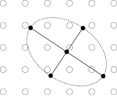
By expanding the matrix products, we have the following expression: \[ ({\frac{du}{dx}}^2 + {\frac{dv}{dx}}^2) {\Delta u}^2 + (\frac{du}{dx}\cdot \frac{du}{dy} + \frac{dv}{dx} \cdot \frac{dv}{dy})2\Delta x \Delta y + ({\frac{du}{dy}}^2+{\frac{dv}{dy}}^2){\Delta y}^2 = 0 \] Hence the parameters \(A, B, C\) of the ellipse is given as: \[ A \cdot {\Delta u}^2 + 2B \cdot \Delta x \Delta y + C \cdot {\Delta y}^2 = 0 \] where: \[ A = {\frac{du}{dx}}^2 + {\frac{dv}{dx}}^2 \\ B = \frac{du}{dx}\cdot \frac{du}{dy} + \frac{dv}{dx} \cdot \frac{dv}{dy} \\ C = {\frac{du}{dy}}^2+{\frac{dv}{dy}}^2 \] Therefore, take \((u_0, v_0)\) as the (projected) center of sampling, we can do gaussian weighted average of each pixel in an area, i.e. \[ \text{Color}(u_0, v_0) = \frac{\sum_{\Delta u, \Delta v} \text{weight}(\Delta u, \Delta v) \cdot \text{Color}(u+\Delta u, v+\Delta v)}{\sum_{\Delta u, \Delta v}\text{weight}(\Delta u, \Delta v)} \] where the weight is given as follows: \[ \text{weight}(\Delta u, \Delta v) = A\cdot {\Delta u}^2 + B \cdot \Delta u\Delta v + C \cdot \Delta v^2 \]
Question Left for Readers
Usually, we require the new basis \(\vec{uv}_i\), i.e. the columns of linear transform \(J\), to be orthogonal. Do we need to do Gram-Schmidt normalization on the vectors \(\vec{uv}_i\)?
(The answer is, No! Think about it~)
Result Gallery
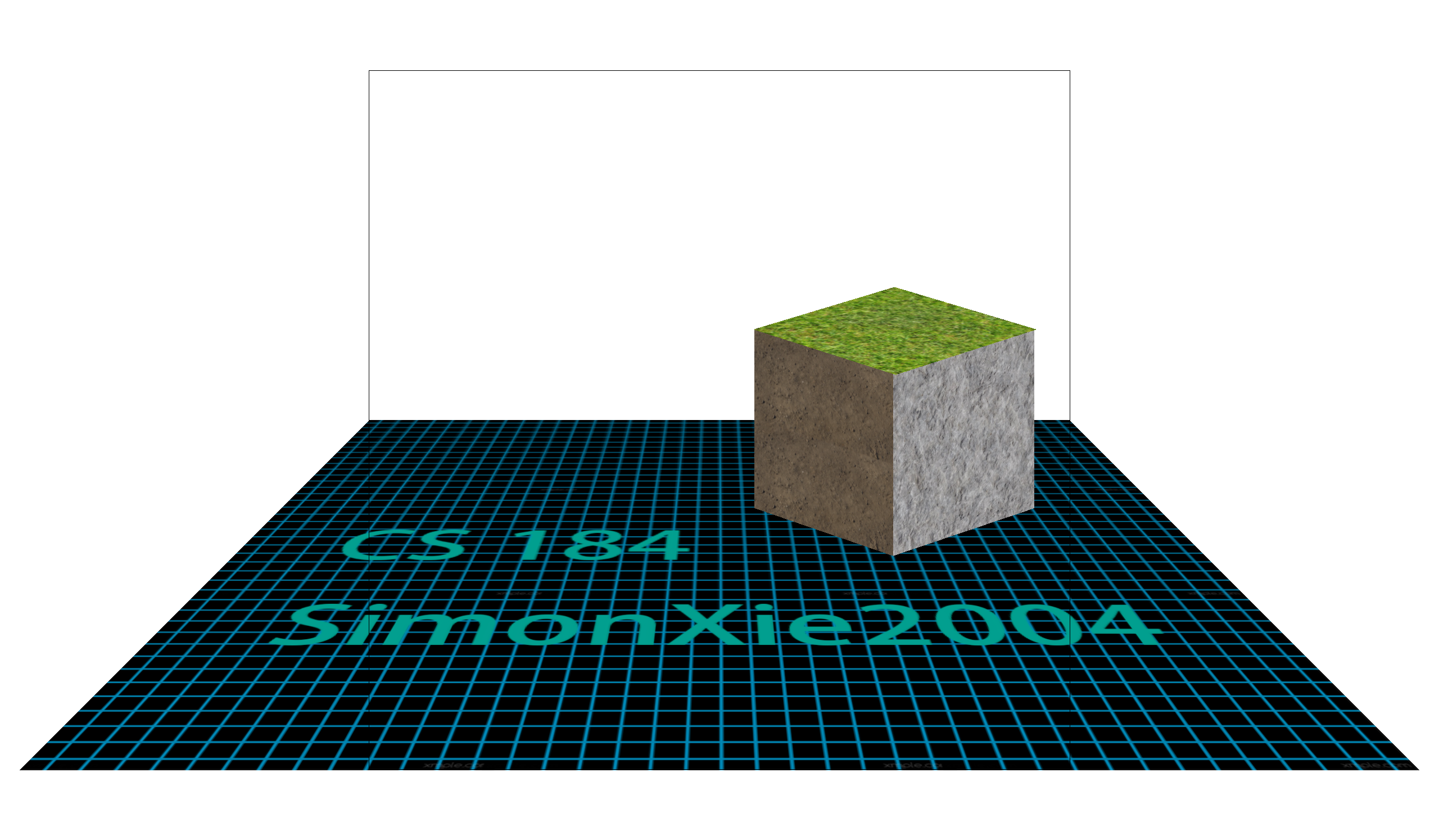
Here are my render results. Pay attention to the distant part of the ground plane and the top surface of the block. You can zoom-in by clicking on the image.
|

|
| Bilinear Pixel + Bilinear Level + MSAA1x | Bilinear Pixel + EWA Filtering + MSAA1x |
My Code
1 | // Inside namspace CGL |