
Overview
This is my implementation of a rasterizer, with core features of:
- Super-fast rasterization* algorithm with line scanning (instead of bounding-box based methods)
- Multithread rendering* with OpenMP
- Antialiasing support (maximum of MSAAx16 on each pixel)
- Perspective Transforms* support and correct texture sampling
- Trilinear Sampling support (bilinear interpolation & mipmap on texture)
- Elliptical Weighted Average (EWA) Filtering* support (on texture sampling)
Terms marked with an asterisk (*) indicate my bonus implementations.
For more detailed mathematical derivation of EWA Filtering,
Please refer to my blog: Mathematical Derivation of EWA Filtering
Task 1: Rasterizing Triangles
Keep takeaways: line-scanning method, openMP parallelization.
In this part, we rasterize triangles by line-scanning method. This is a method optimized from bounding-box scanning method, which avoids doing line-tests with those pixels that are not in the bounding box.
Method Overview
Here is a short pseudocode about how this method works:
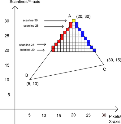
- Sort each vertex such that they satisfy \(y_0 < y_1 < y_2\)
- For each vertical coordinate \(j\) in range \([y_0, y_2]\):
- Calculate left and right boundary* as \([x_{\text{left}}, x_{\text{right}}]\)
- For each horizontal coordinate \(i\) in range \([x_{\text{left}}, x_{\text{right}}]\):
- Fill color at coordinate \((i, j)\) on screen space.
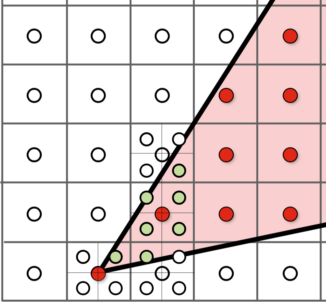
*Kindly reminder: You should be extremely careful when calculating left and right boundary. The lines may cover half (or even less) of a pixel; However, when doing MSAA antialiasing, you still must calculate the sub-pixel here. Hence, my recommend is doing two edge interpolations (using both \(y\) and \(y+1\) instead of solely \(y+0.5\)), and use the widest horizontal range you can find.
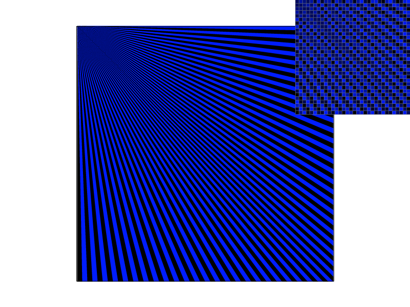
Here is a comparison of line-scanning based method and bounding-box based ones.
|
|
| line-scanning rasterization (faster) | bounding-box rasterization |
Method Optimization
Taking intuition from Bresenham's Line Algorithm, we
can optimize the double for-loop in rasterize_triangle
function by replacing the float variables i, j
by int objects. This will avoid the time-consuming float
operations.
Also, this facilitates another optimization, i.e.
parallelized rendering. To further improve the speed, I
additionally added openmp support, and parallelized
pixel-sampling process.
Performance Comparison
By adding clock() before/after svg.draw()
call, I recorded the time difference of the rendering process. Here is a
performance comparison of some methods:
| Method | B-Box | Line-Scanning |
Line-Scanning (with OpenMP) |
|---|---|---|---|
| Render Time (ms) | 80ms | 45ms | 18ms (fastest) |
REMARK: I used the final version with texture to test performance.
Render target:
.\svg\texmap\test1.svg, same as the result gallery in Task 5Resolution: 800 * 600; Use num_thread: 12
CPU: Intel Core Ultra 9 185H (16 cores (6*P, 8*E, 2*LPE), 22 threads)
Result Gallery
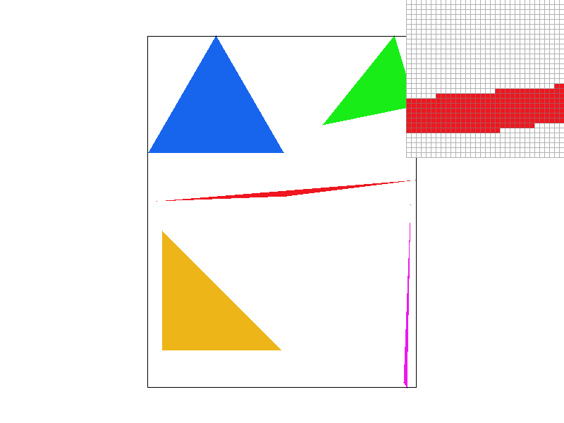
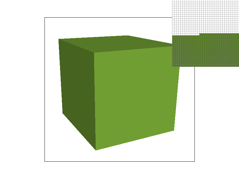
We can show some examples of rasterization result. As we can see, without antialiasing, the edges of triangles remain jaggy. In the following sections, we will use MSAA to solve this problem.
|
|
| thin triangles | a cube |
Task 2: Anti-Aliasing
Key takeaways: MSAA sampling method, screen buffer data structure.
As seen before, we have a jaggy result from the previous part. Hence, we add MSAA antialiasing in this subpart.
Method Overview
MSAA is the simplest method to smooth edges and reduce visual artifacts. By sampling multiple points per pixel and averaging the colors, we alleviate the jaggies.
Here is a pseudocode of my modification to the previous rasterization function. (Grey parts remains same; Blue parts are newly added.)
- Sort each vertex such that they satisfy \(y_0 < y_1 < y_2\)
- For each vertical coordinate \(j\) in range \([y_0, y_2]\):
- Calculate left and right boundary as \([x_{\text{left}}, x_{\text{right}}]\)
- For each horizontal coordinate \(i\) in range \([x_{\text{left}}, x_{\text{right}}]\):
- For each sub-pixel in pixel \((i, j)\)
- If sub-pixel \((i + dx, j
+ dy)\) in triangle:
- Set
screen_buffer[i, j, r]^ to colorc
- Set
- Else:
- Do nothing*
- If sub-pixel \((i + dx, j
+ dy)\) in triangle:
- For each sub-pixel in pixel \((i, j)\)
^Note:
ris the r-th sub-pixel in pixel \((i, j)\), which will be temporarily saved in screen buffer.*Kindly Reminder: You mustn't do anything sub-pixel \((i+dx, j+dy)\) if it is NOT in the current triangle. Because if it was in another triangle previously (but not the current one), the rendered color will be overwritten.
Key Structure/Function
Also, we must do the following modification to the previous data
structure of screen_buffer and resolve_buffer
function. Here are the modifications:
| screen_buffer | resolve_buffer | |
| Previously | Array of W*H | Array of WHS (S=samples per pixel) |
| Currently | Directly render screen_buffer[i, j] | Render avg(screen_buffer[i, j, :]) |
Result Gallery
Here is a table that organizes and compares the rendered images under different MSAA configurations.
| MSAA x1 | MSAA x4 | MSAA x9 | MSAA x16 |
|---|---|---|---|

|
|

|

|
|
|
|
|
- The first row displays the middle section of a red triangle, highlighting the jagged edges and how they are progressively smoothed by increasing levels of MSAA.
- The second row presents a more extreme case: a zoomed-in view of a very skinny triangle corner. In the first image, some triangles appear disconnected, as the pixels covered by the triangle occupy too little area to be rendered. However, with higher MSAA settings, the true shape of the triangle becomes fully visible.
Here is the most extreme case: an image full of degenerate triangles. My implementation successfully passes this test.
| MSAA x1 | MSAA x16 |
|---|---|
|
|
|
|
Task 3: Transforms
Key takeaways: homogeneous coordinates, transform matrices
In this section, we define the 2D transform matrices to support 2D Transforms. The transforms are done in homogeneous coordinates, mainly because translation is not a linear operator, while matrix multiplication is.
Here we define the 2D Homogeneous coordinates as \([x, y, 1]\). Hence the transforms can be
expressed by the following matrices: \[
\text{Translate:}
\begin{bmatrix}
1 & 0 & tx \\
0 & 1 & ty \\
0 & 0 & 1
\end{bmatrix}, \quad
\text{Scaling:}
\begin{bmatrix}
s_x & 0 & 0 \\
0 & s_y & 0 \\
0 & 0 & 1
\end{bmatrix}, \quad
\text{Rotation:}
\begin{bmatrix}
\cos\theta & -\sin\theta & 0 \\
\sin\theta & \cos\theta & 0 \\
0 & 0 & 1
\end{bmatrix}
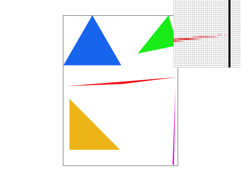
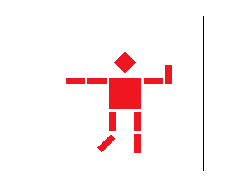
\] Here is my_robot.svg, depicting a stick figure
raising hand, drawn using 2D transforms.
Also, I have implemented perspective transforms by calculating the four-point, 8 DoF matrix, i.e. solving the following 4-point defined (\(ABCD \rightarrow A'B'C'D'\)) transform: \[ \begin{pmatrix} x_1 & y_1 & 1 & 0 & 0 & 0 & -x_1 x_1' & -y_1 x_1' \\ 0 & 0 & 0 & x_1 & y_1 & 1 & -x_1 y_1' & -y_1 y_1' \\ x_2 & y_2 & 1 & 0 & 0 & 0 & -x_2 x_2' & -y_2 x_2' \\ 0 & 0 & 0 & x_2 & y_2 & 1 & -x_2 y_2' & -y_2 y_2' \\ \vdots & \vdots & \vdots & \vdots & \vdots & \vdots & \vdots & \vdots \\ x_N & y_N & 1 & 0 & 0 & 0 & -x_N x_N' & -y_N x_N' \\ 0 & 0 & 0 & x_N & y_N & 1 & -x_N y_N' & -y_N y_N' \end{pmatrix} \cdot \begin{pmatrix} a \\ b \\ c \\ d \\ e \\ f \\ g \\ h \end{pmatrix} = \begin{pmatrix} x_1' \\ y_1' \\ x_2' \\ y_2' \\ \vdots \\ x_N' \\ y_N' \end{pmatrix} \] Here is an example result:
Task 4: Barycentric Coordinates
Key takeaways: area explanation & distance explanation of barycentric coords.
Now we are adding more colors to a single triangle. Try imagining a triangle with 3 vertices of different colors, what will it look like inside? This is the intuition of barycentric coordinates: interpolating attributes of 3 vertices inside a triangle. This algorithm is quite useful in multiple ways, for example, shading.
Explanation 1: Proportional Distances
The first explanation comes from the intuition of distance: we have
the params defined as follow for interpolation and use the similar
construction for other coordinates: \[
\alpha = \frac{L_{BC}(x, y)}{L_{BC}(x_A, y_A)}
\]
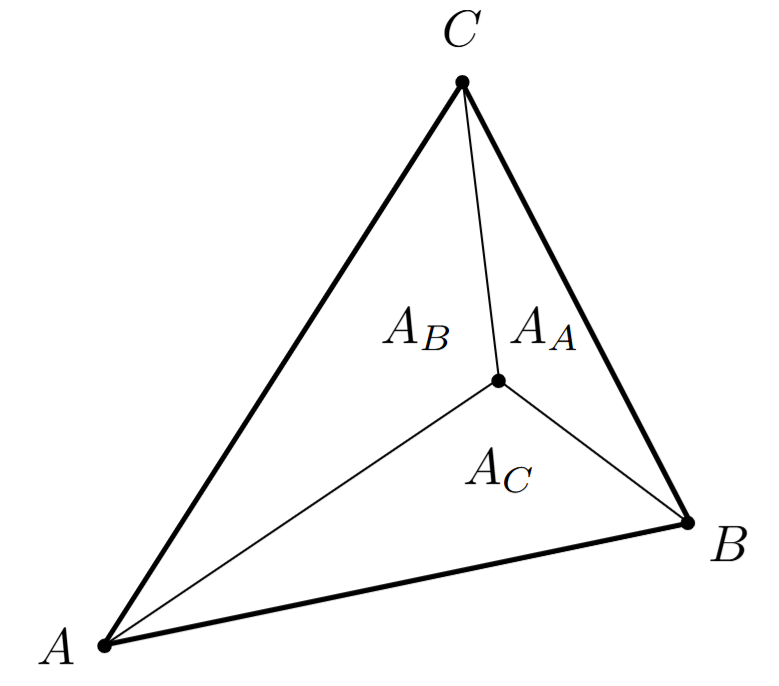
Explanation 2: Area Interpolation
The second explanation comes from area: we have the params defined as
proportions of area (and use similar construction for other
coordinates): \[
\alpha = \frac{A_A}{A_A + A_B + A_C}
\]
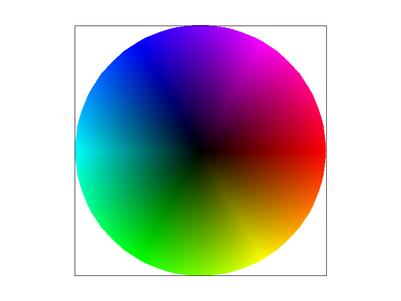
Result Gallery
With barycentric coordinates, we can interpolate any point inside a triangle, even we only have the vertex colors! Here is a example result combined of multiple triangles:
Task 5: Pixel Sampling
Key takeaways: nearest / bilinear / elliptical weighted average sampling
In this section, I implement three different sampling methods, i.e. nearest, bilinear and elliptical weighted average (EWA) filtering (which is one of the anisotropic sampling methods), and compare their performance.
Method Overview
Mainly speaking, sampling is the process of back-projecting \((x, y)\) coordinate to \((u, v)\) space, and selecting a texel to represent pixel \((x, y)\)'s color. However, the back-projected coordinates aren't always integers, which aren't given any color information (since texels only provide color information on integer grids). Hence we need sampling methods. Here are the methods that are implemented:
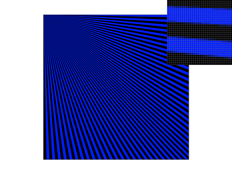
- Nearest Sampling selects the closest texel to the given sampling point without any interpolation, which is fast and efficient but can result in blocky, pixelated visuals.
- Bilinear sampling improves image quality by using the weighted average between the four nearest texels surrounding the sampling point. However, it can still introduce blurriness when scaling textures significantly.
- EWA Filtering Sampling (EWA) filtering is a high-quality texture sampling method. It considers multiple texels in an elliptical region, weighting them based on their distance to the sampling point using a gaussian kernel. This method reduces aliasing and preserves fine details, but it is computationally expensive compared to nearest and bilinear sampling.
Here is a comparison of the three methods:
|
|
|
| Nearest Sampling | Bilinear Sampling | EWA Filtering |
Perspective Transforms: An Exception
When applying barycentric coordinates in rasterization, we typically assume that interpolation in screen space is equivalent to interpolation in the original 2D space. However, when a perspective transform is applied, this assumption breaks down because perspective projection distorts distances non-linearly. This means that linearly interpolating attributes (e.g., color, texture coordinates) in screen space does not match the correct interpolation in world space.
But there is still solution: we can first back-project the triangle vertices to the original space. When sampling screen-pixel \((i, j)\), we can also do the same back-project and then interpolate. Here is the fixed pseudocode:
- Back-Project triangle vertices \(A, B, C\) back to \(A', B', C'\)
- ... inside rasterization loop, sampling at \((i, j)\)
- Back-Project screen-space pixel \((i, j)\) back to \((i', j')\)
- Calculate barycentric interpolation using \(A', B', C'\), \((i', j')\)
- Pass \(\alpha, \beta, \gamma\) to texture sampling function...
Here is a comparison of wrong implementation and correct implementation:
|
|
Result Gallery
The first two standard methods' results are as follows:
| MSAA x1 | MSAA x16 | |
| Nearest Sampling |

|
|
| Bilinear Sampling |

|

|
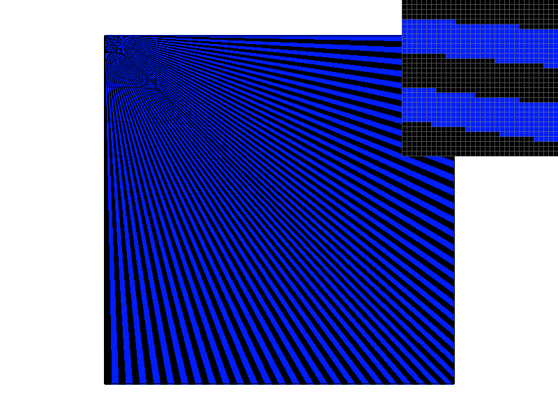
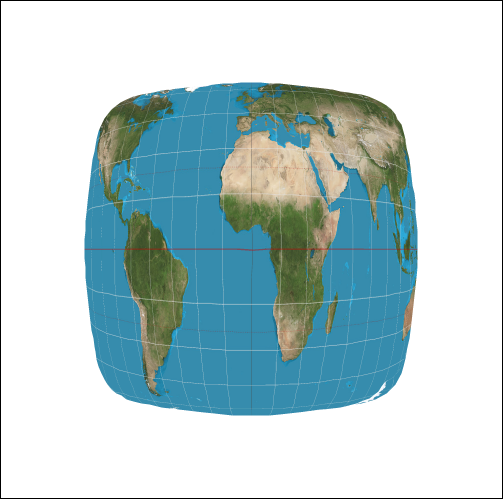
The differences are obvious. In the cases that the texels are quite sparse or sharp (for example, the meridians in the map), nearest sampling will create a lot of disconnected subparts which looks quite like jaggies. However, with bilinear sampling, the disconnected parts appear connected again.
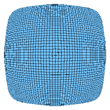
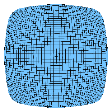
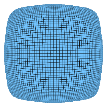
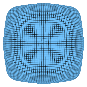
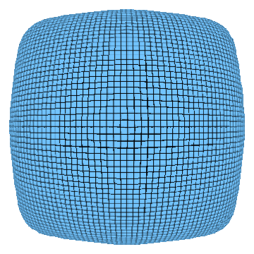
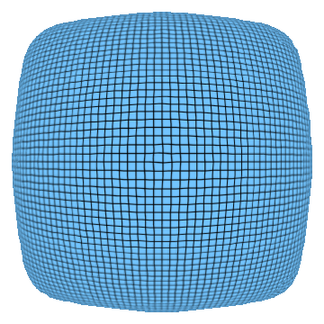
Also, the render result of anisotropic filtering (EWA) method is provided as follows. Pay attention to the distant part of the ground plane and the top surface of the block. You can zoom-in by clicking on the image.
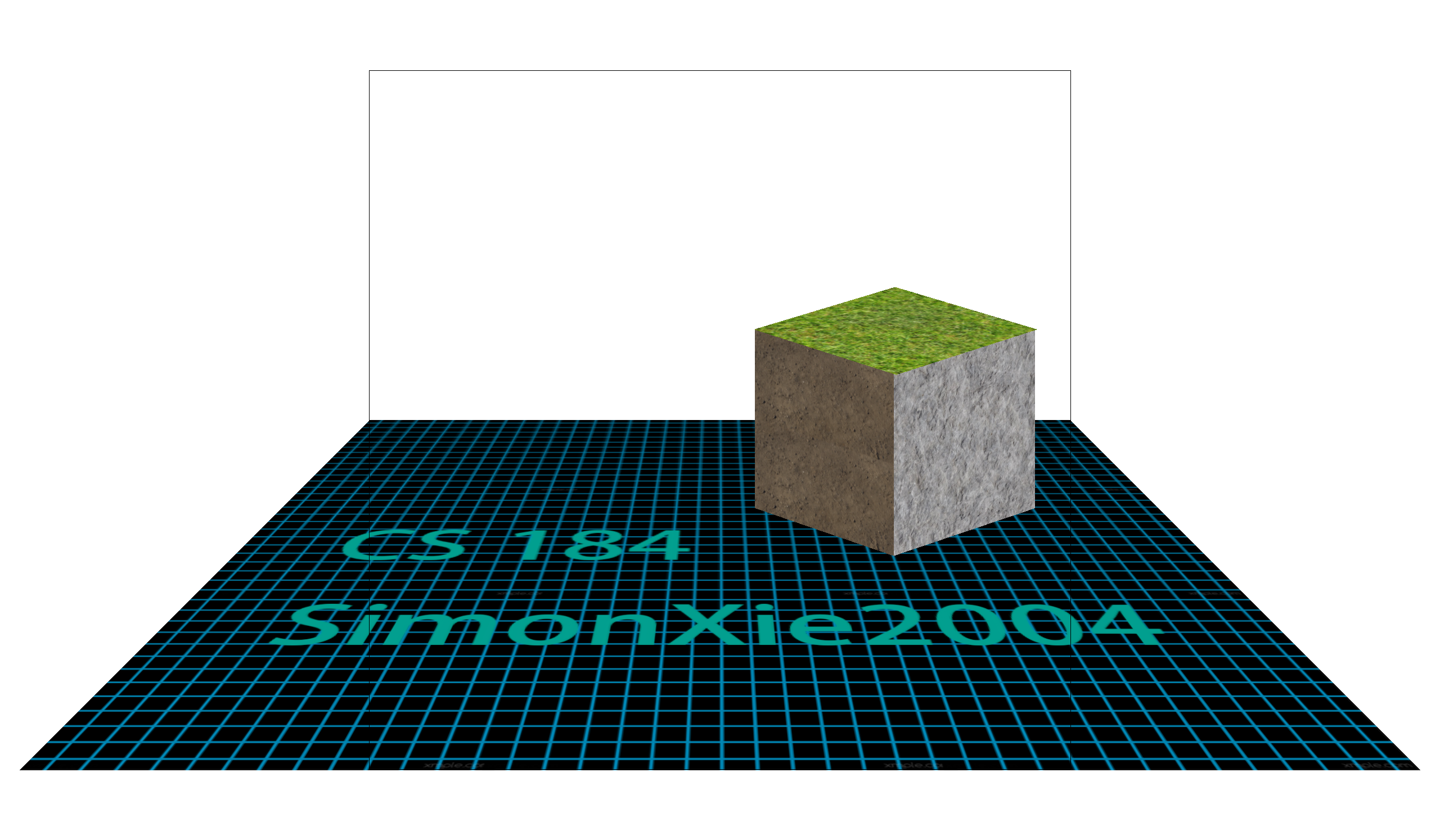
|

|
| Bilinear Pixel + Bilinear Level + MSAA1x | Bilinear Pixel + EWA Filtering + MSAA1x |
For more detailed mathematical derivation of EWA Filtering,
Please refer to my blog: Mathematical Derivation of EWA Filtering
Task 6: Level Sampling
Key takeaways: calculating \(\frac{\partial dx}{\partial du}\), mip level L, mipmaps
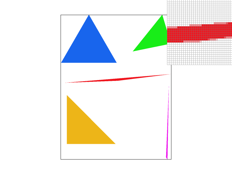
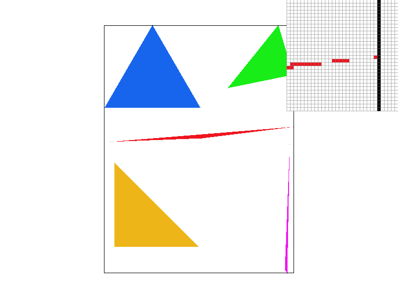
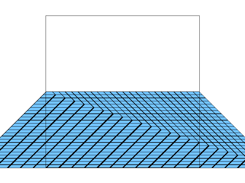
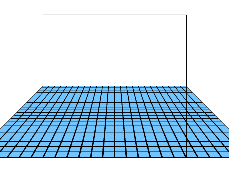
The concept of level sampling naturally arises from the previous problem. When sampling from texture space, a single pixel may cover a large area, making it difficult to accurately represent the texture. Simply sampling the nearest 1–4 pixels can lead to unrepresentative results, while manually computing the area sum is inefficient. To address this issue, we use level sampling techniques, such as mipmapping, which enhance both accuracy and efficiency.
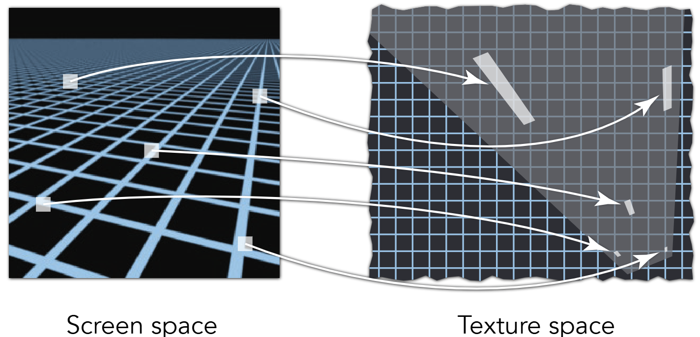
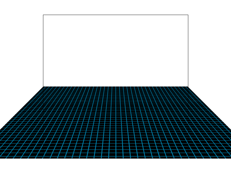
Example: different pixels have different texture space footprint
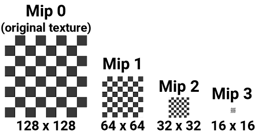
Mipmap Overview
Here we implement mipmap, which is a list of downsampled texture, each at progressively lower resolutions. When rendering, the appropriate mipmap level is chosen based on the texture-space pixel size, ensuring that a pixel samples from the most suitable resolution. This reduces aliasing artifacts and improves performance by avoiding unnecessary high-resolution texel averaging.
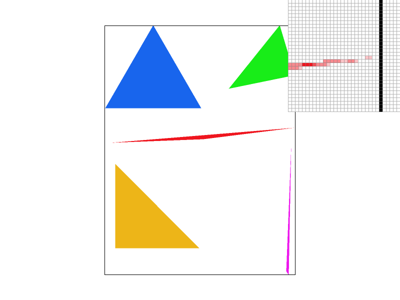
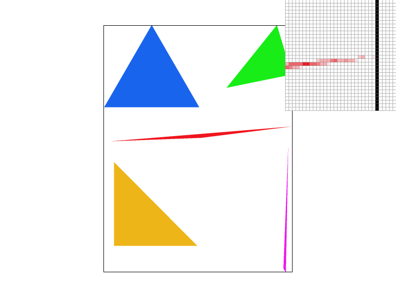
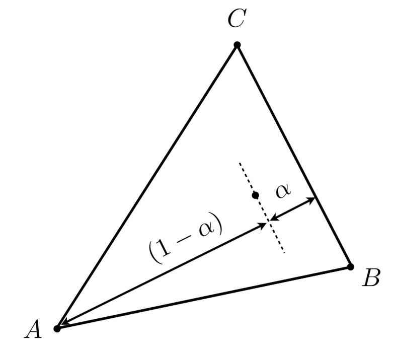
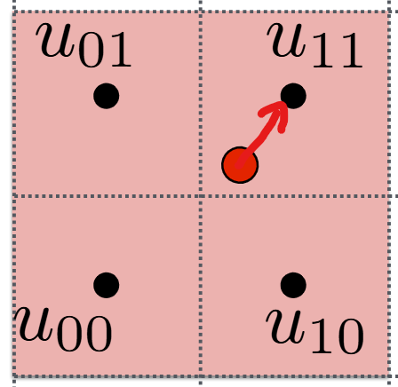
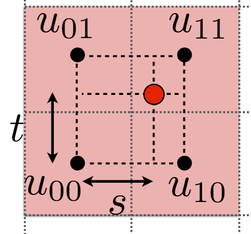
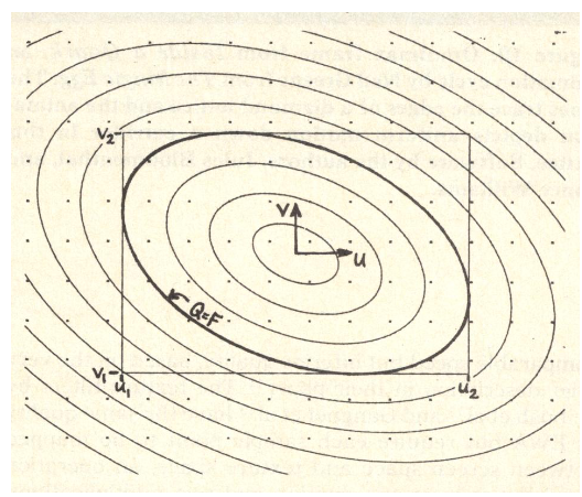
Here is an image intuitive of \(L\) and partial derivatives. We inspire from it to learn how to choose the corresponding mip level to sample texture from.
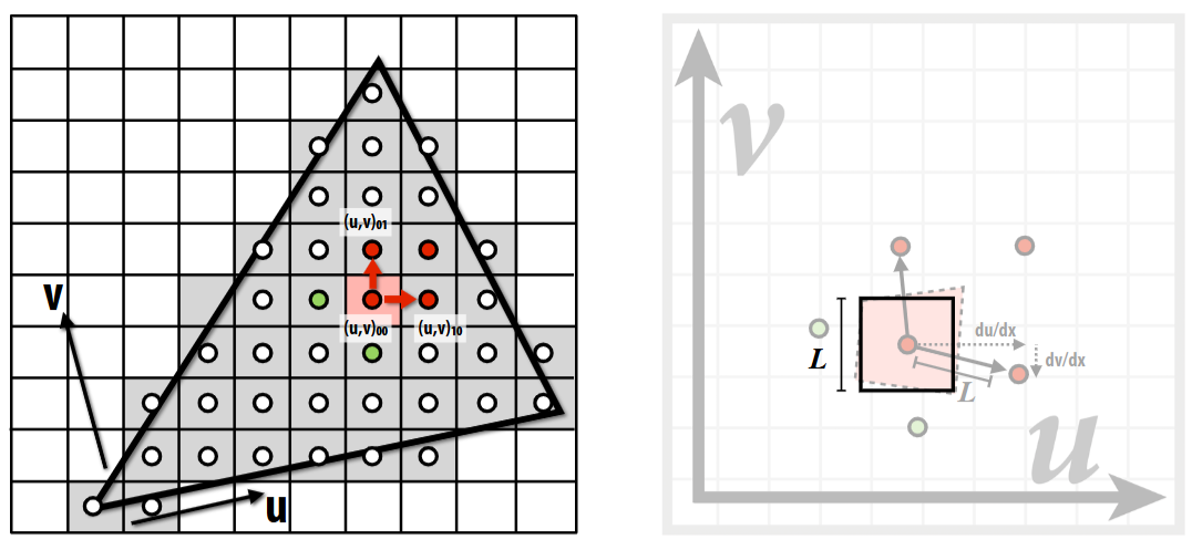 Therefore, we can calculate the level
\(L\) as follows: \[
L = \max \left( \sqrt{\left(\frac{du}{dx}\right)^2 +
\left(\frac{dv}{dx}\right)^2}, \sqrt{\left(\frac{du}{dy}\right)^2 +
\left(\frac{dv}{dy}\right)^2} \right)
\] where \(\frac{du}{dx}\) is
calculated as follows:
Therefore, we can calculate the level
\(L\) as follows: \[
L = \max \left( \sqrt{\left(\frac{du}{dx}\right)^2 +
\left(\frac{dv}{dx}\right)^2}, \sqrt{\left(\frac{du}{dy}\right)^2 +
\left(\frac{dv}{dy}\right)^2} \right)
\] where \(\frac{du}{dx}\) is
calculated as follows:
- Calculate the uv barycentric coordinates of \((x, y)\) \((x+1, y)\) \((x, y+1)\)
- Calculate the corresponding uv coordinates \((u_0, v_0)\) \((u_1, v_1)\) \((u_2, v_2)\)
- Hence \(\frac{du}{dx} = u_1 - u_0\), and the rest are the same.
Level Blending Overview
By blending between mip levels (trilinear filtering), we can achieve smoother transitions and further enhance visual quality. If a level is calculated as a float, we use linear-interpolation, which samples from both levels and do a weighted average. This reduces the artifacts created by sudden change of level of detail.
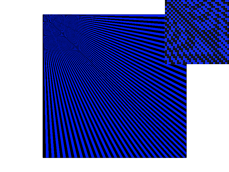
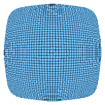
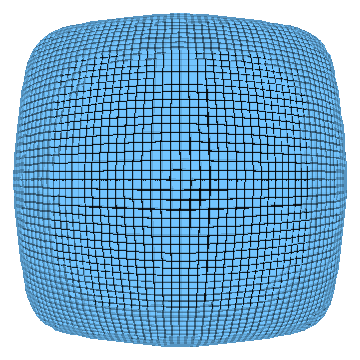
Result Gallery
|
Level/Pixel Sampling |
Nearest | Bilinear | EWA |
|---|---|---|---|
| L_zero |
|
|
|
| L_nearest |
|
|
|
| L_linear |
|
|
|
Final Discussion
- Speed. Better methods are more time-consuming.
Sorted by render time:
- Pixel sampling: EWA >> Bilinear > Nearest
- Level sampling: L_bilinear >> L_nearest > L_zero
- Antialiasing: MSAAxN cost N times time.
- Memory.
- Pixel sampling doesn't cost more memory.
- Level sampling: Mipmap costs 2x texture space memory.
- Antialiasing requires \(r\) times memory buffer, but can be done in-place.