Implementing NeRF

 2024/11/29 

UC Berkeley CV Project 6 - Implementing Neural Radiance Fields

Part I: Fit a Neural Field to a 2D Image

Introduction

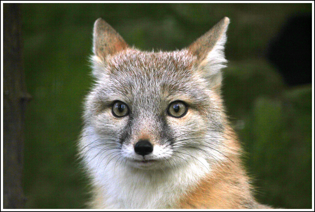
We know that we can use a Neural Radiance Field (NeRF) (\(F:\{x,y,z,\theta, \phi\}\rightarrow\{r,g,b,\sigma\}\)) to represent a 3D space. But before jumping into 3D, let's first get familiar with NeRF using a 2D example. In fact, since there is no concept of radiance in 2D, the Neural Radiance Field falls back to just a Neural Field (\(F:\{u,v\}\rightarrow \{r,g,b\}\)) in 2D, in which \(\{u,v\}\) is the pixel coordinate. Hence, in this section, we will create a neural field that can represent a 2D image and optimize that neural field to fit this image.

MLP: We start from the following MLP structure, but the number of hidden layers (Linear 256 in the graph) is configurable as parameter num_hidden_layers. We will show the effect of different num_hidden_layers later.
Sinusoidal Positional Encoding (PE): PE is an operation that you apply a serious of sinusoidal functions to the input cooridnates, to expand its dimensionality (See equation 4 from this paper for reference). Note we also additionally keep the original input in PE, so the complete formulation is \[ PE(x) = \left[ x, \sin\left( 2^0 \pi x \right), \cos\left( 2^0 \pi x \right), \cdots, \sin\left( 2^{L-1} \pi x \right), \cos\left( 2^{L-1} \pi x \right) \right] \]

Experiments

For the following results, we let:

Learning Rate = 1e-3
Number of Hidden Neurons = 256
Batch Size = "full image" (meaning that each batch is consisted of all pixels from the original image)

And, the following params are subject to different experimental values:

N = num_hidden_layers
L = maximum positional encoding power

N=3 L=10
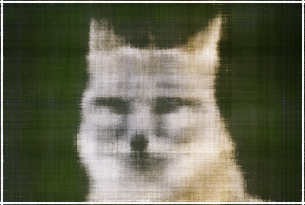
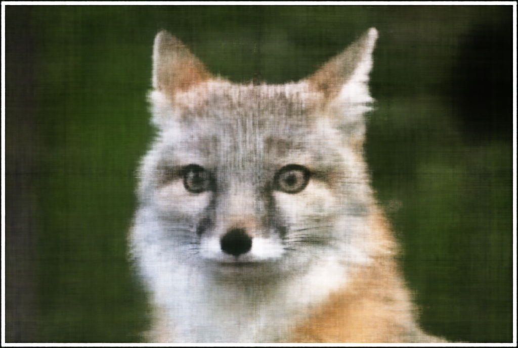
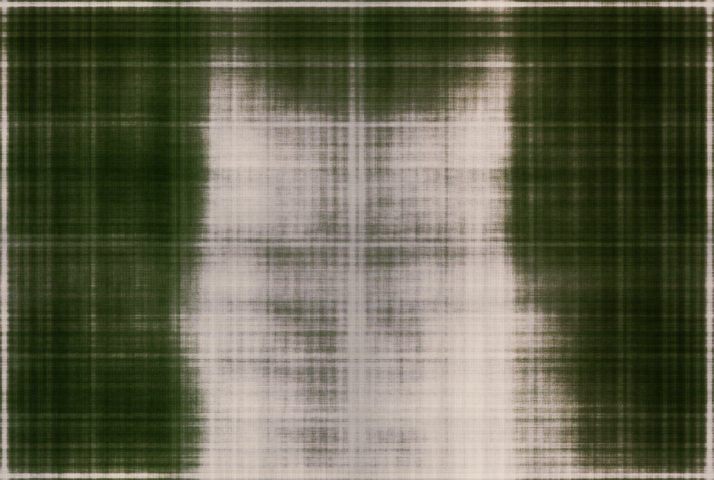
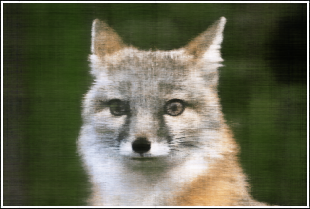
N=3 L=10	Epoch=64, PSNR=16.72	Epoch=128, PSNR=21.30	Epoch=512, PSNR=25.58	Epoch=4096, PSNR=28.43
N=5 L=20
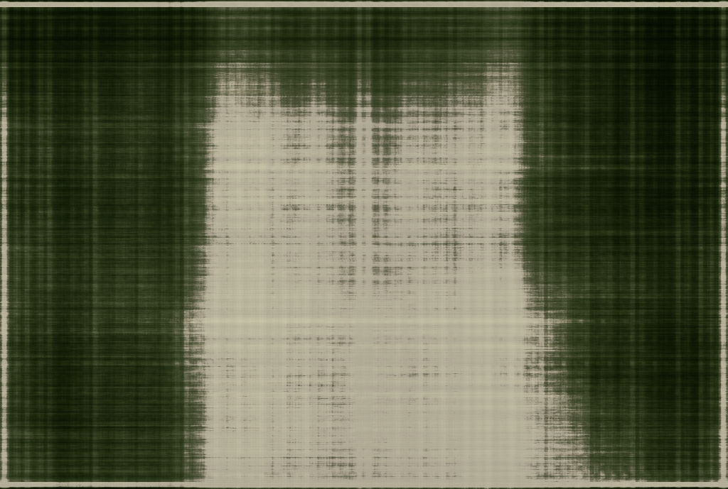
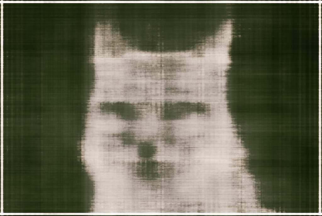
N=5 L=20	Epoch=64, PSNR=15.97	Epoch=128, PSNR=19.95	Epoch=512, PSNR=25.39	Epoch=4096, PSNR=29.76

PSNR
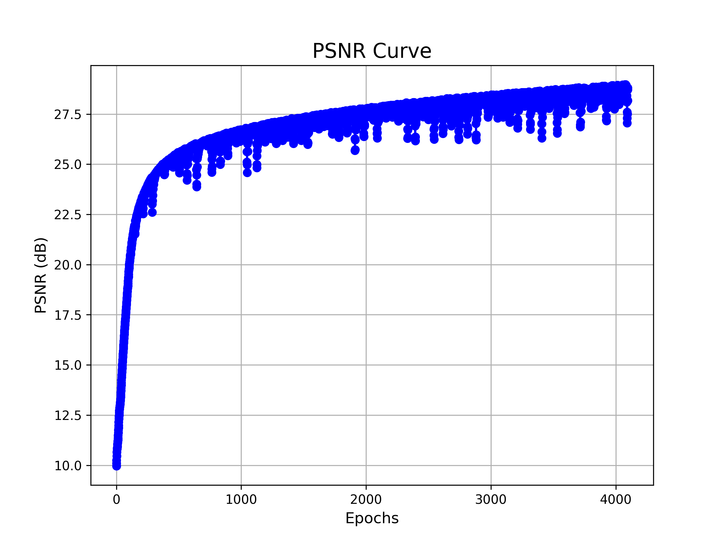
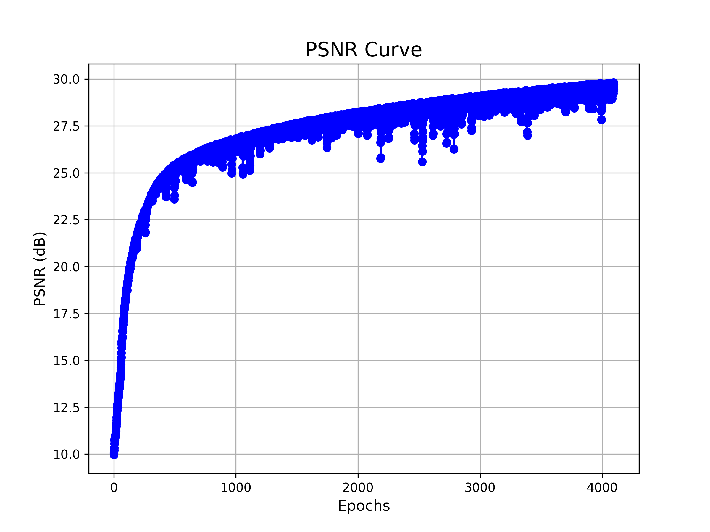
PSNR	PSNR Curve for config 1 (N=3, L=10)	PSNR Curve for config 2 (N=5, L=20)

The results align well with our expectations: Larger networks and deeper positional encodings make convergence more challenging, but ultimately lead to better performance.

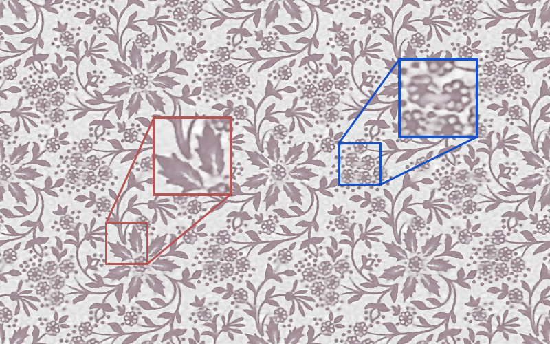
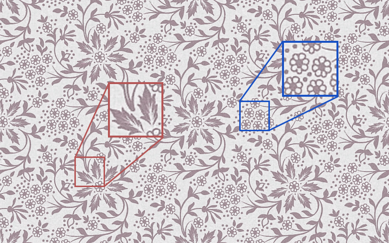
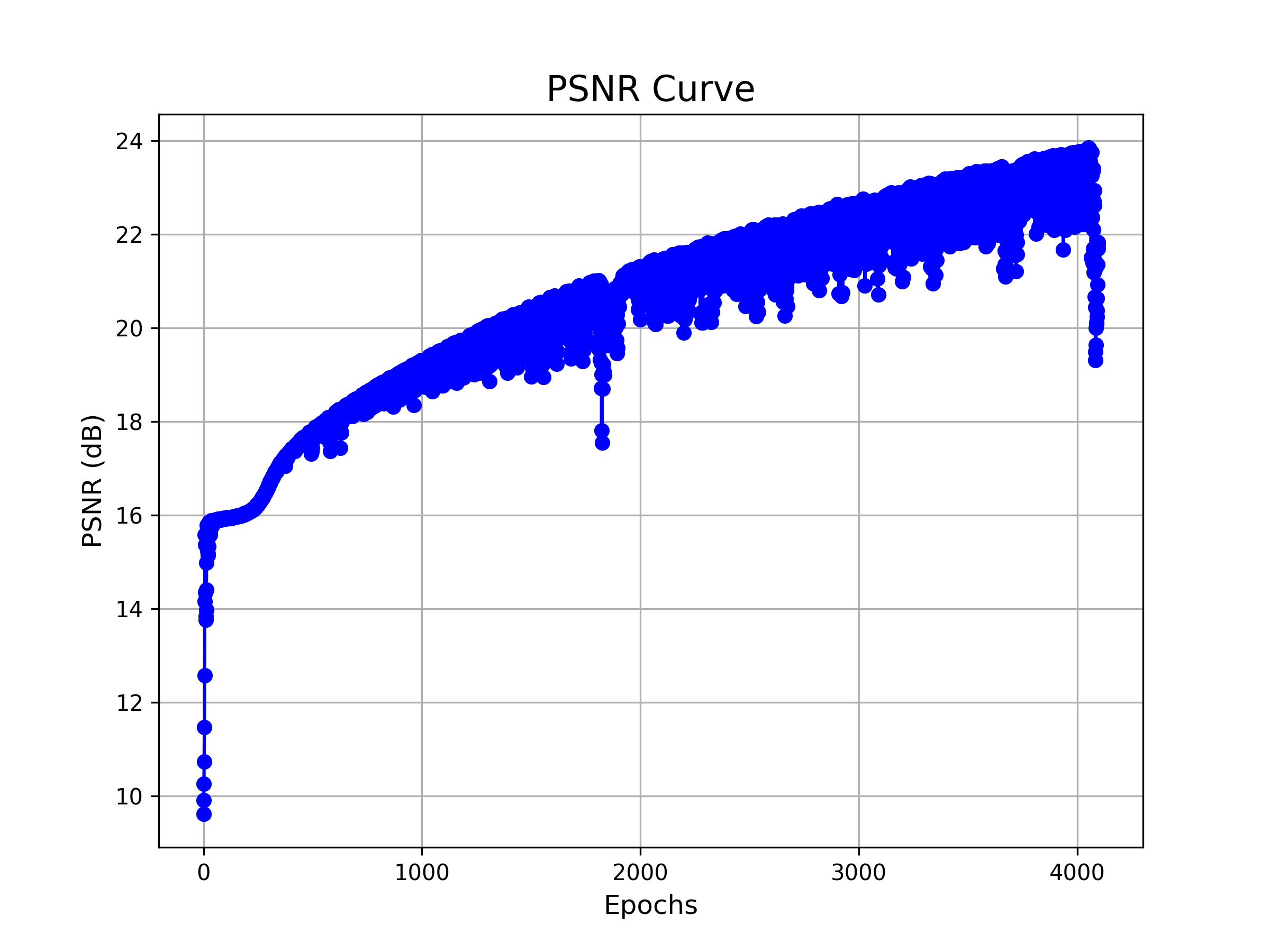
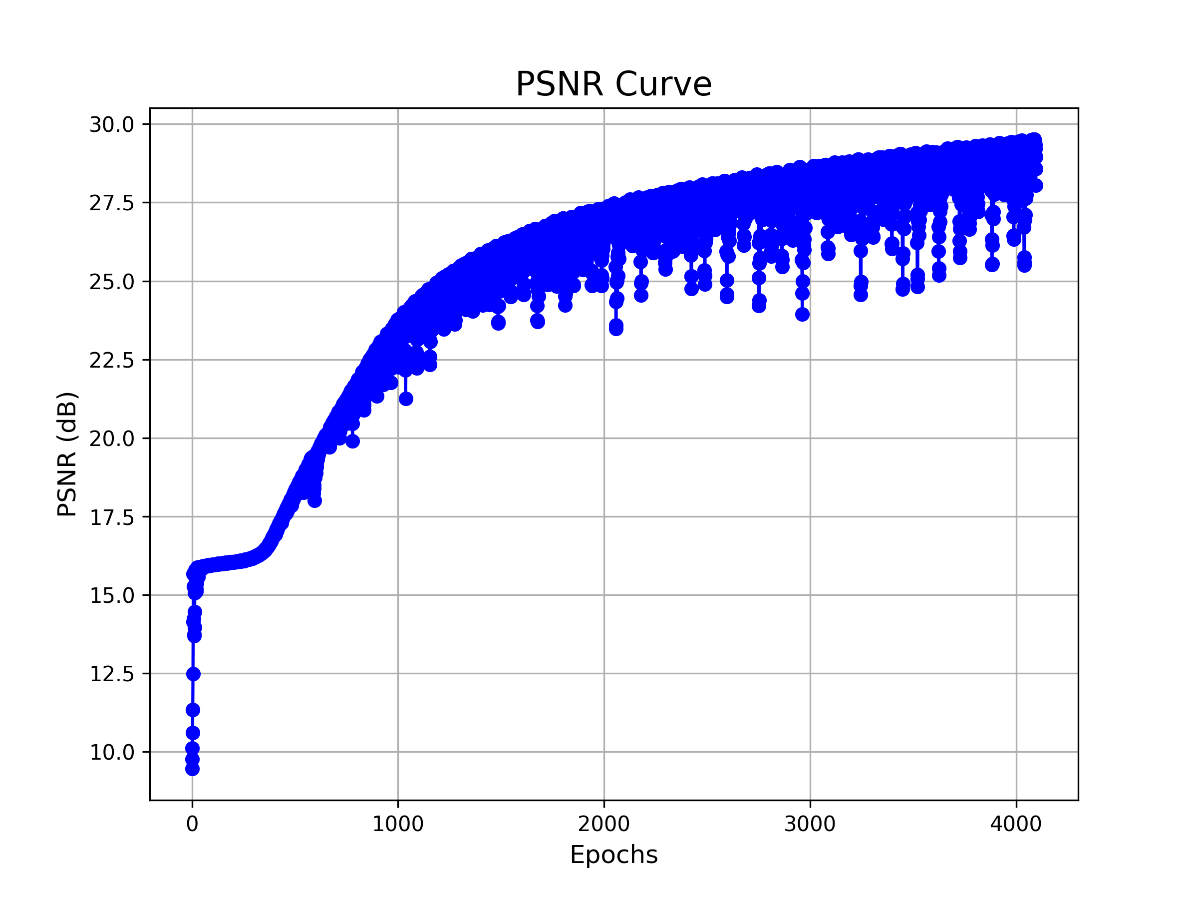
Furthermore, we aim to demonstrate the effectiveness of our positional encoding. To achieve this, we conduct an ablation experiment to visualize the differences, where both images have same neural network but different positional encoding powers.

texture

N=3
N=3	L=5, PSNR=22.46	L=20, PSNR=28.76

PSNR
PSNR	PSNR Curve for config 1 (L=5)	PSNR Curve for config 2 (L=20)

Part II: 3D Neural Radiance Field!

Introduction

Neural Radiance Fields (NeRF) is a deep learning framework introduced for generating photorealistic 3D scenes from a sparse set of 2D images. NeRF models the scene as a continuous volumetric scene representation, where a neural network is trained to predict the color and density of points in 3D space. It has shown success in synthesizing realistic novel views of a scene, particularly for photo-realistic rendering, by leveraging the power of neural networks.

Dataloader

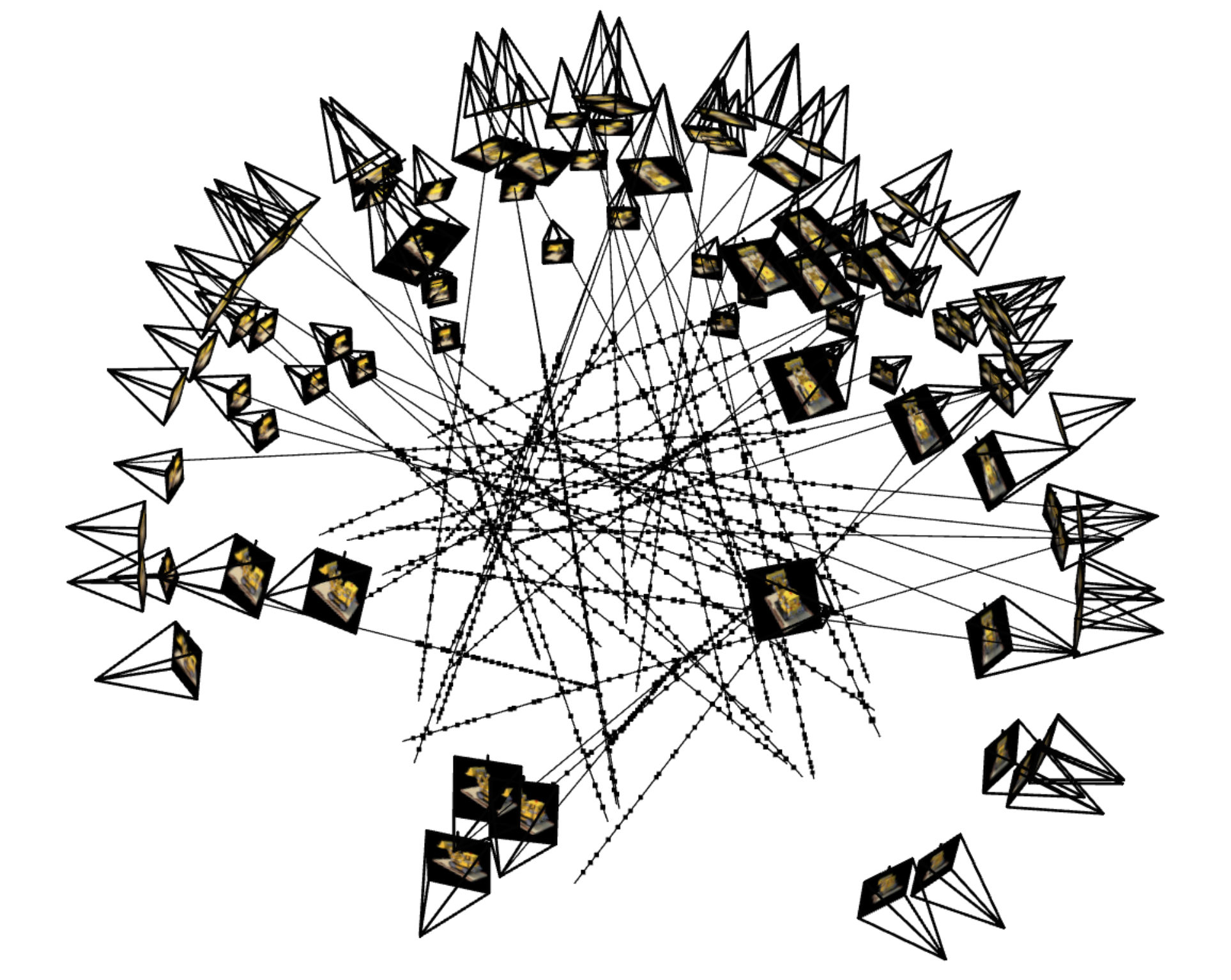
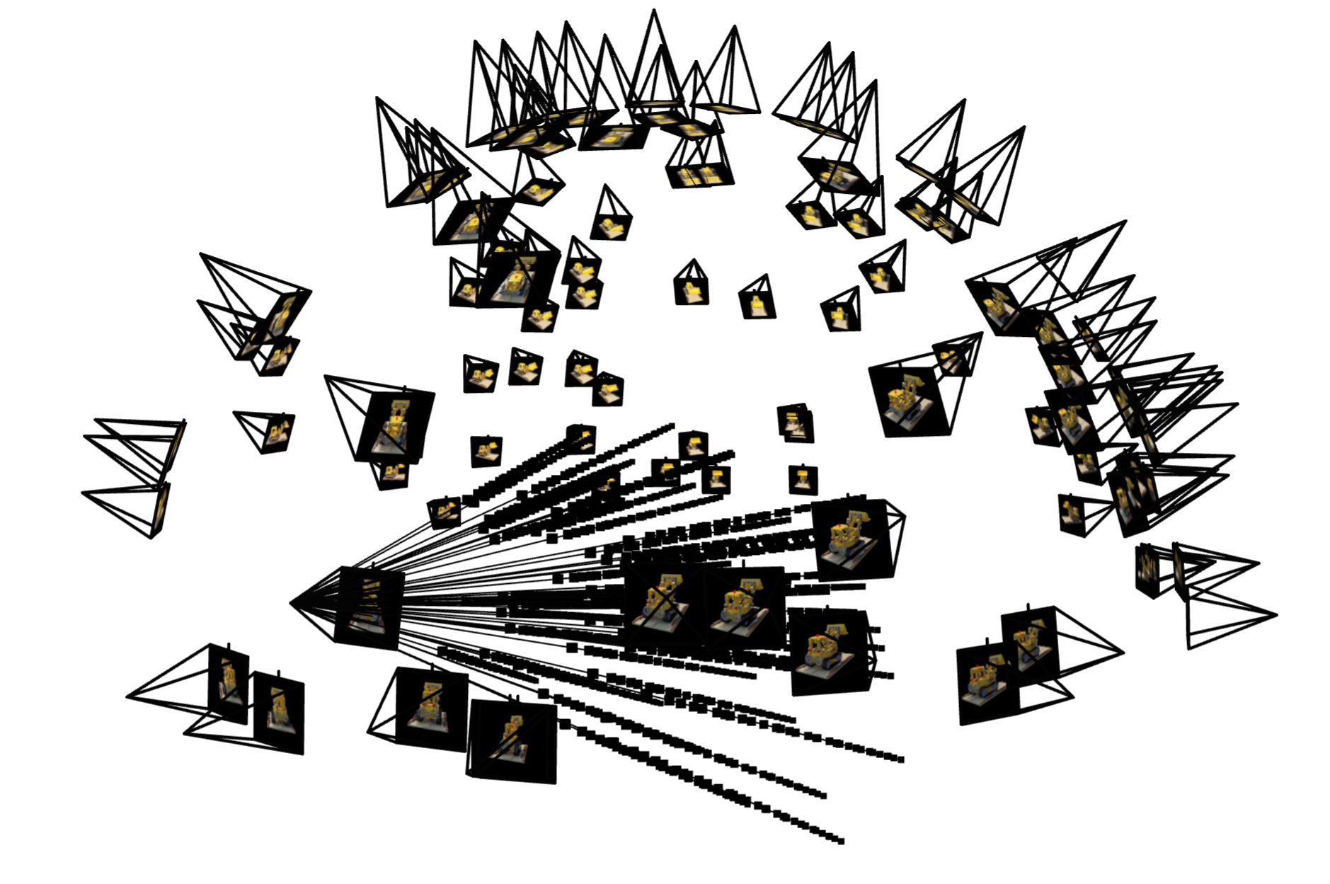
In NeRF, the core idea is that we want to compute how light travels through a 3D scene by casting rays from a camera into the scene. Each ray represents a potential view of a point in the scene, and it passes through the 3D volume. (Hence, this requires that we know each camera's position and looking-direction, i.e. the cameras are calibrated)

Camera rays: During training, rays are cast from the camera's viewpoint through each pixel of the image, into the scene. Each pixel in the image corresponds to one ray in 3D space. The parameter \(r_o\) and \(r_d\) can be calculated as follows: \[ r_o = \mathbf{t} \\ r_d = \frac{\mathbf{X_w} - \mathbf{r_o}}{\| \mathbf{X_w} - \mathbf{r_o} \|} \]

(Suppose that the calibrated extrinsics are c2w matrices)

Here’s a simple illustration of this step:

Scene Representation (MLP)

NeRF represents a 3D scene as a continuous function that predicts the color and density at any given 3D point, parameterized by spatial coordinates and viewing directions. Specifically, a neural network \(f_{\theta}\) learns to predict the radiance (color) and volume density at a point \(\mathbf{x} = (x, y, z)\) and view direction \(\mathbf{d}\): \[ f_\theta(\mathbf{x},\mathbf{d})=(\hat{C},\sigma) \] where \(\hat{C}\) is the color and \(\sigma\) is the volume density.

Here, we implement the following network architecture as our NeRF scene representation. Remark that by concatenation of x in the middle of linear layers, we can let the network "remember" the positional information.

Volumn Rendering

The core volume rendering equation is as follows: \[ C(\mathbf{r}) = \int_{t_n}^{t_f} T(t) \cdot \sigma(\mathbf{r}(t)) \cdot \mathbf{c}(\mathbf{r}(t), \mathbf{d})dt \text{, where } T(t) = \exp(-\int_{t_n}^t\sigma(\mathbf{r}(s)))ds \] This fundamentally means that at every small step \(dt\) along the ray, we add the contribution of that small interval \([t,t+dt]\) to that final color, and we do the infinitely many additions if these infintesimally small intervals with an integral.

The discrete approximation (thus tractable to compute) of this equation can be stated as the following: \[ \hat{C}(\mathbf{r}) = \sum_{i=1}^N T_i(1 - \exp(-\sigma_i\delta_i))\mathbf{c}_i \text{, where } T_i = \exp(-\sum_{j=1}^{i-1}\sigma_j\delta_j) \]

Experiments


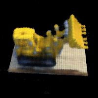
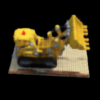
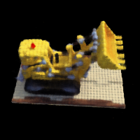
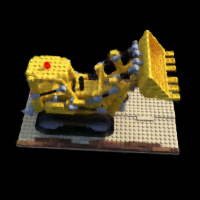
Epoch 1024	Epoch 2048	Epoch 4096	Epoch 8192	Epoch 40960

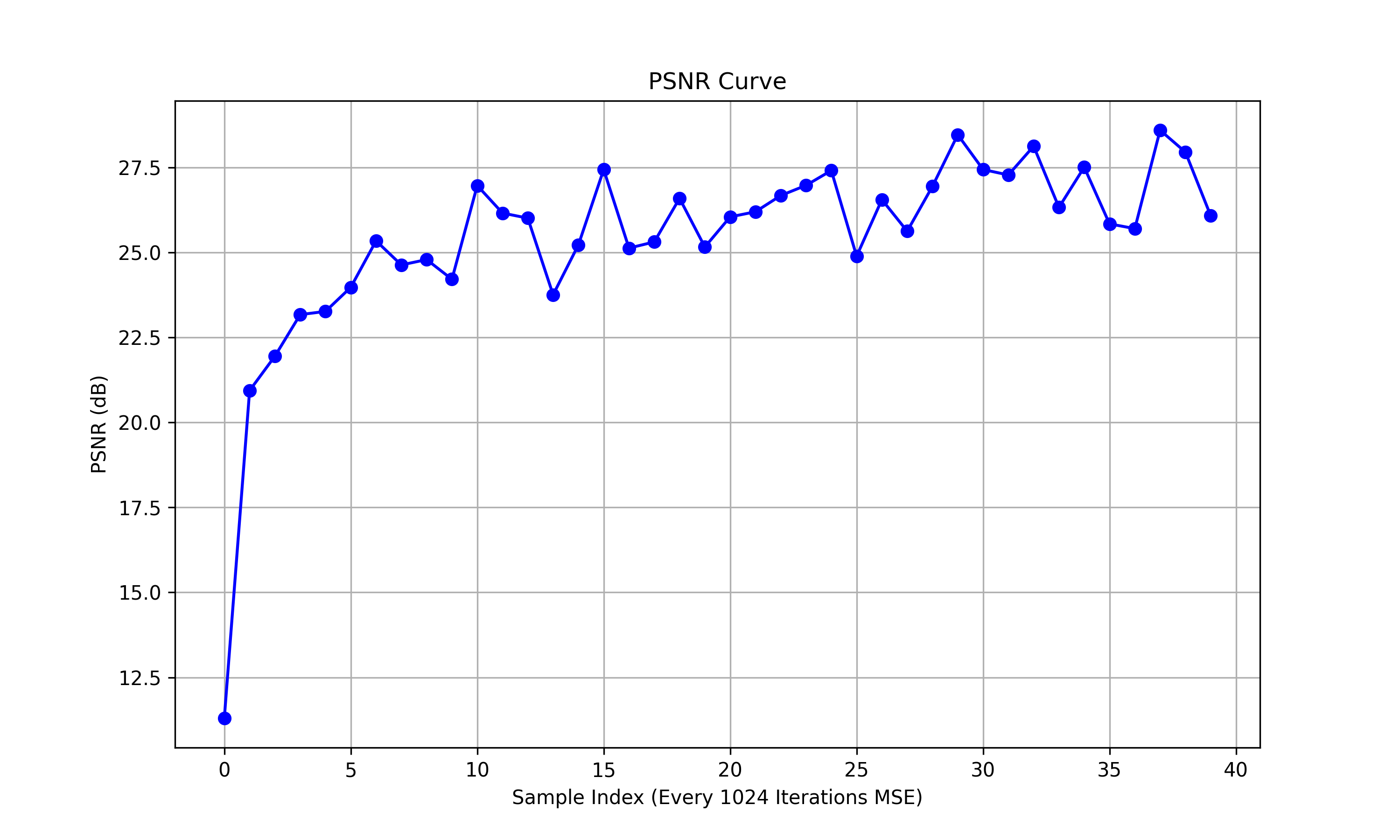
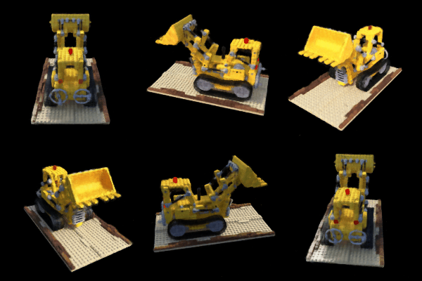
And the final result on test set is:

B&W: Bells and Whistles

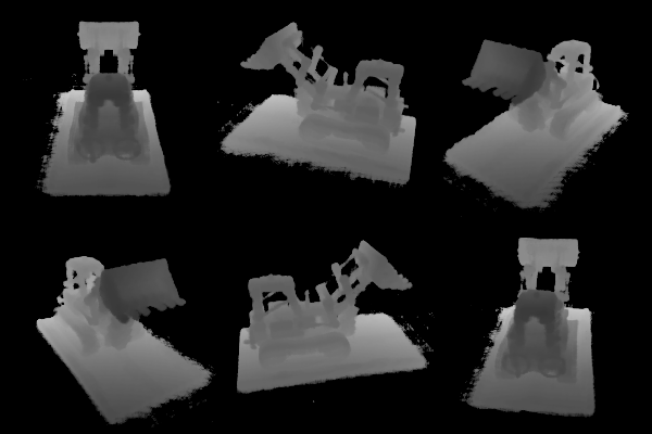
NeRF computes depth by integrating the expected distance along rays through a scene. Each sampled point along a ray contributes to the depth value based on its density and the accumulated transmittance. This can also be understood as an "expectation" of ray depth. Specifically:

\[ \text{Depth} = \sum_{i=1}^N T_i \cdot \sigma_i \cdot z_i \cdot \Delta t_i \]

where:

\[ T_i = \prod_{j=1}^{i-1} \exp(-\sigma_j \cdot \Delta t_j) \]

This process ensures depth corresponds to the most opaque or highly weighted regions in the scene, aligning with rendered colors.