UC-Berkeley 24FA CV Project 4a & 4b:
Creating panorama images by correspondence detecting, projective warping, resampling and compositing them together.
A simpler reproduction of Multi-Image Matching using Multi-Scale Oriented Patches
Project 4a: Manual Image Panorama
Creating panoramas by manually registering corresponding points
Shoot and Digitize pictures
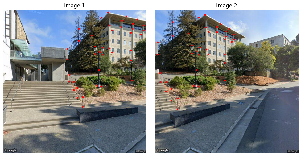
First, we retrieve some images surrounding memorial glade @ Berkeley.
These images have same center of projection (COP) and different looking directions.
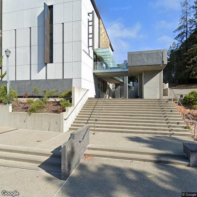
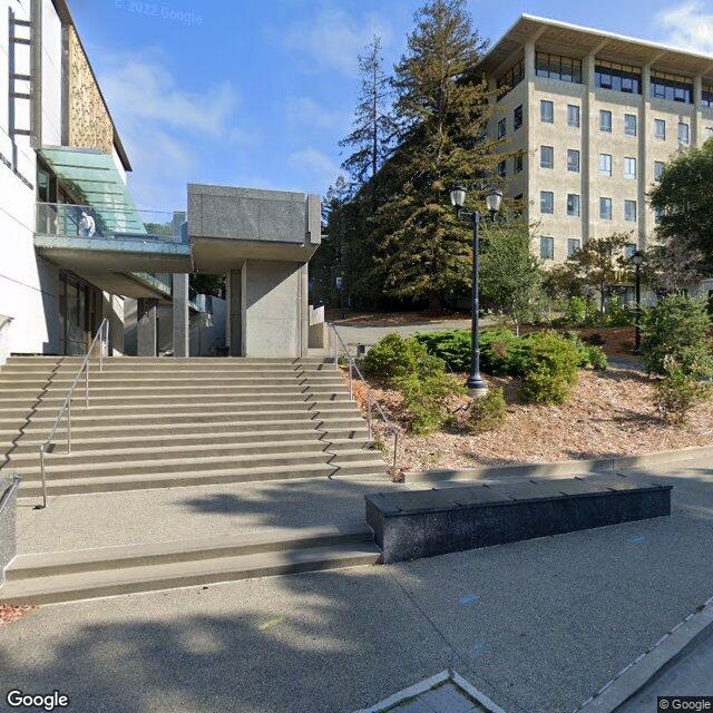
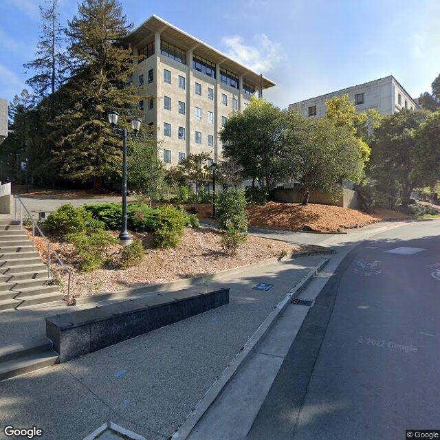
Then we define the following corresponding points manually:
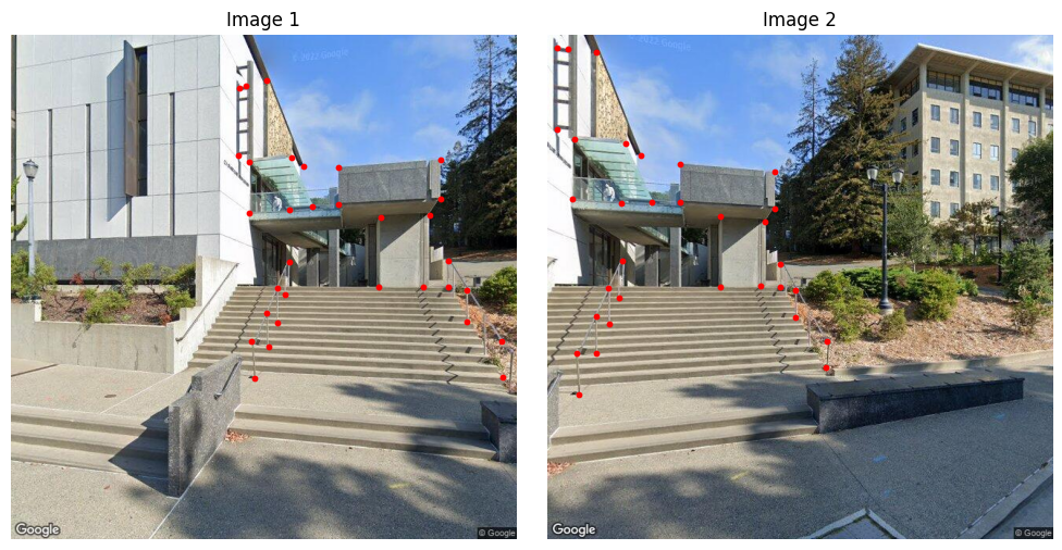
Recover Homographies
The transform between images is basically a projection transform with 8 degree of freedoms. This can be written as: \[ H \mathbf{p} = \mathbf{p}' \] where: \[ H = \begin{pmatrix} a & b & c \\ d & e & f \\ g & h & 1 \end{pmatrix} \]
Expanding it out would get: \[ \begin{aligned} w'x' &= a x + b y + c \\ w'y' &= d x + e y + f \\ w' &= g x + h y + 1 \end{aligned} \]
Further expansion (into eight separate variables and a linear system) will result: \[ \begin{pmatrix} x_1 & y_1 & 1 & 0 & 0 & 0 & -x_1 x_1' & -y_1 x_1' \\ 0 & 0 & 0 & x_1 & y_1 & 1 & -x_1 y_1' & -y_1 y_1' \\ x_2 & y_2 & 1 & 0 & 0 & 0 & -x_2 x_2' & -y_2 x_2' \\ 0 & 0 & 0 & x_2 & y_2 & 1 & -x_2 y_2' & -y_2 y_2' \\ \vdots & \vdots & \vdots & \vdots & \vdots & \vdots & \vdots & \vdots \\ x_N & y_N & 1 & 0 & 0 & 0 & -x_N x_N' & -y_N x_N' \\ 0 & 0 & 0 & x_N & y_N & 1 & -x_N y_N' & -y_N y_N' \end{pmatrix} \cdot \begin{pmatrix} a \\ b \\ c \\ d \\ e \\ f \\ g \\ h \end{pmatrix} = \begin{pmatrix} x_1' \\ y_1' \\ x_2' \\ y_2' \\ \vdots \\ x_N' \\ y_N' \end{pmatrix} \]
Thus, we have least square method to solve this over-determined equation.
h = np.linalg.inv(A.T @ A) @ (A.T @ b)ORh, _, _, _ = np.linalg.lstsq(A, b, rcond=None)
Warp the Images
With the projection matrix, we may warp any image 1 to image 2. We implement this by:
- First, project the four corners of image 1 to image 2, defining an
areathat img1 will be projected onto. - Second, rasterize the
area, covering all pixels that img1 will be projected onto. - Third, inversely project all pixels in
areaback to image 1 and sample them bilinearly. This will give us the projected image.
Remark: using
scipy.interpolate.griddatais too slow here since it has to query the whole point set. Hence we can implement the bilinear-interpolation and vectorize it using numpy operations ourselves.- First, project the four corners of image 1 to image 2, defining an
Here is our example result:

Image Rectification
According to project requirements, we should perform "rectification" on image to check if the projection works correctly.
Here is an example:
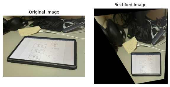
Here we require the ipad in the scene to be rectangular (and hence defined corresponding points on four corners.)
Another example:
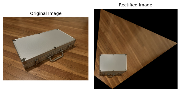
Image Blending
To avoid weird edge artifacts (usually caused by simply covering one image by another),
we develop a method to blend images together with an seamless transition.
First, we generate a mask as follows.
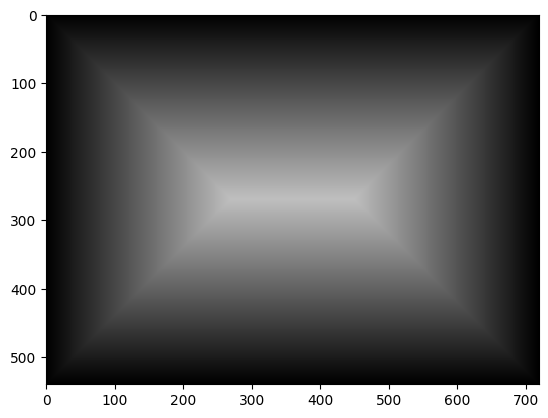
Second, we blend images together according to the mask's values.
For pixels that only the middle image cover, we use its original value.
For pixels that are covered by multiple images, set it to
mask * middle_value + (1-mask) * avg(other_values)Here is an example result:

Ablation study:
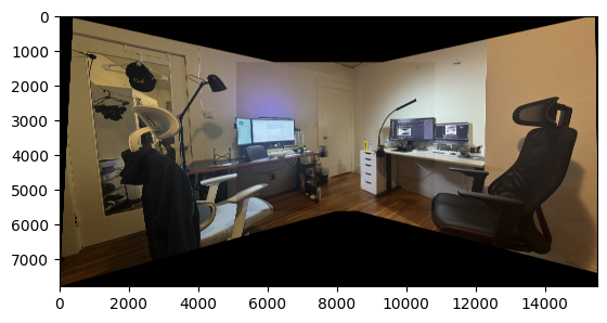
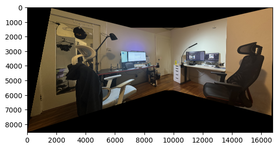
Up: w/o blending; Down: with blending
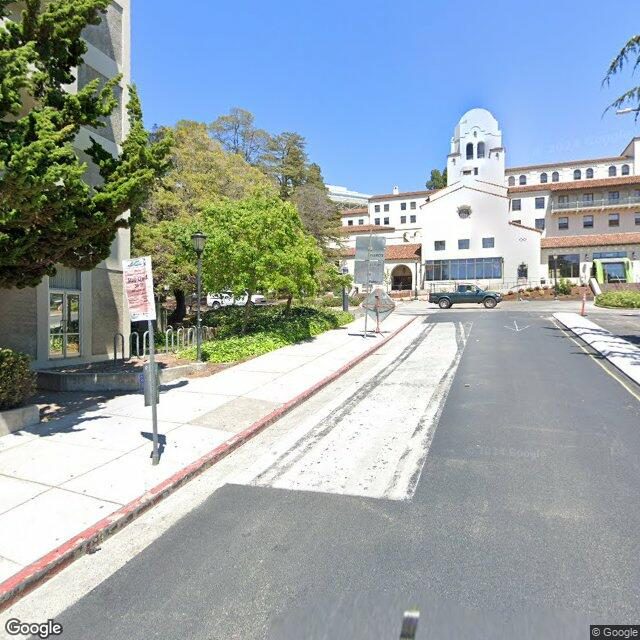
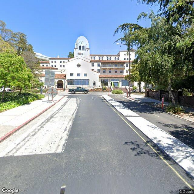
Project 4a: Result Gallery
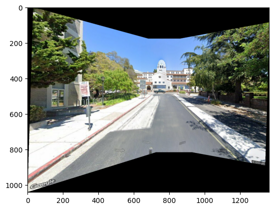
Bancoft St.

|
|
|
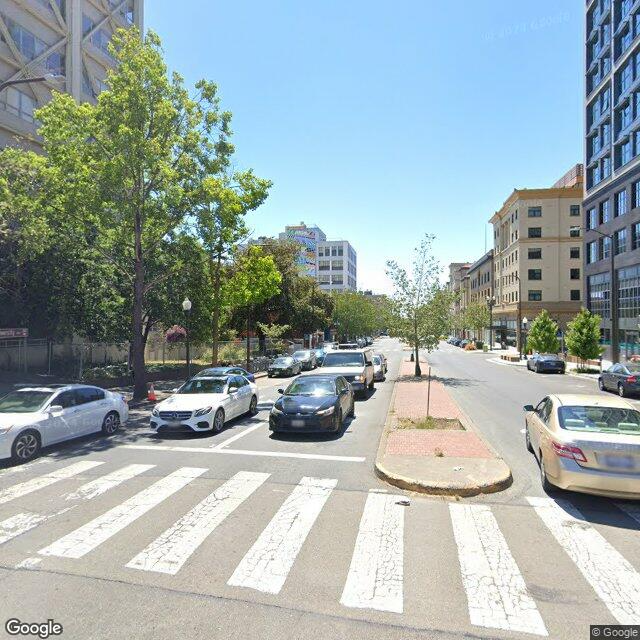
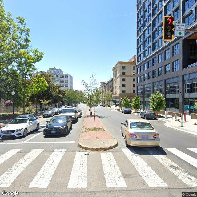
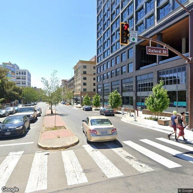
Oxford St.
|
|
|
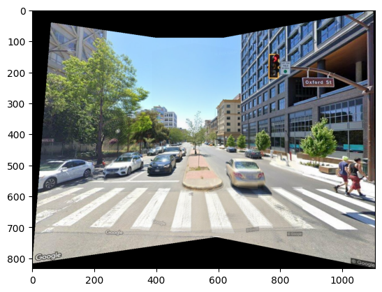
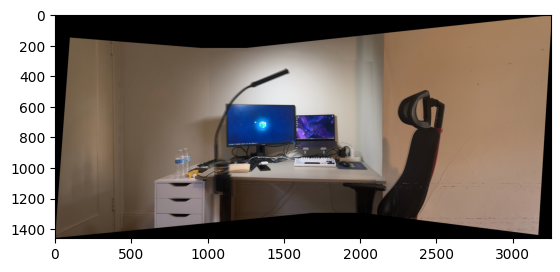
My Home
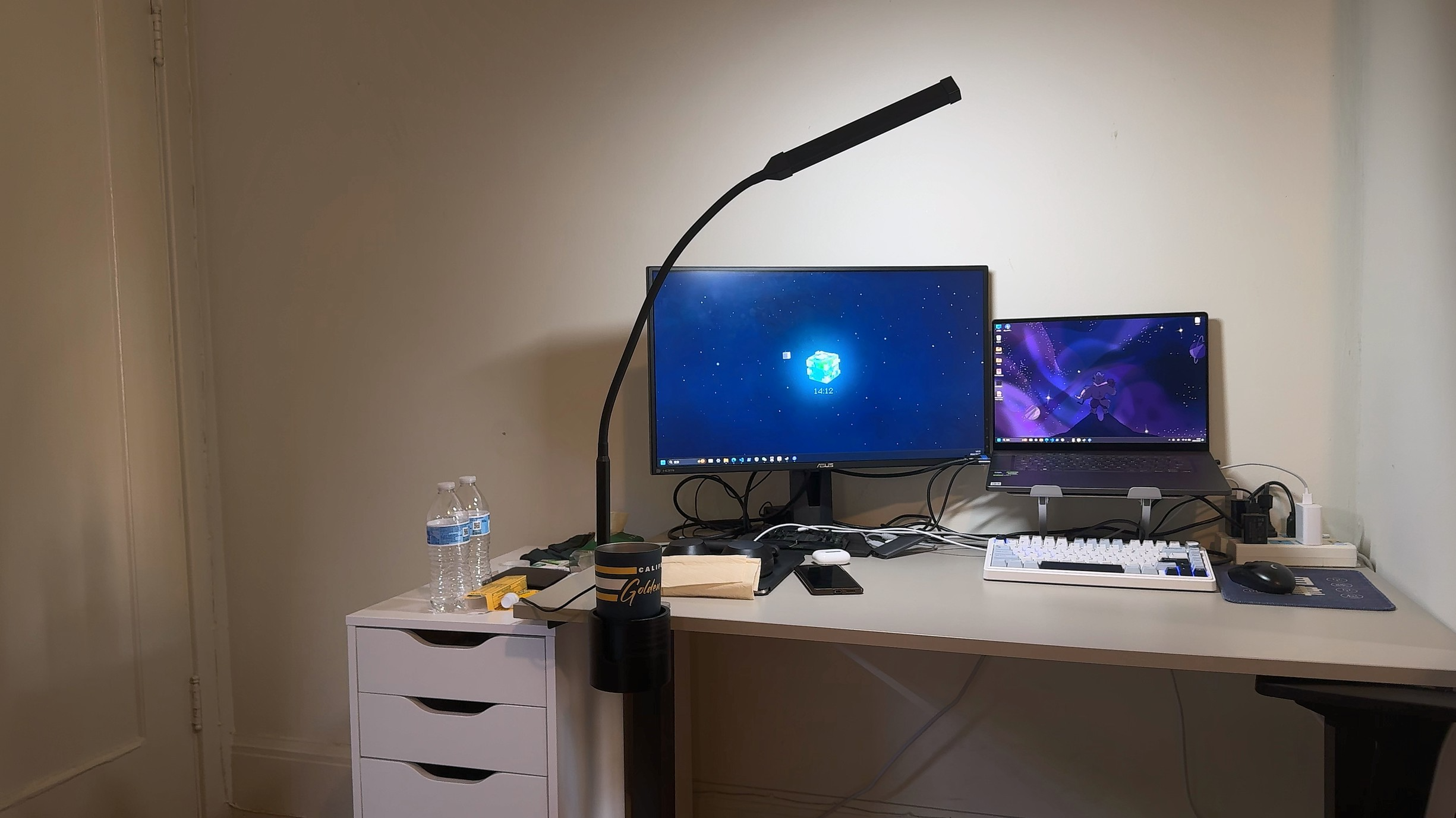
|
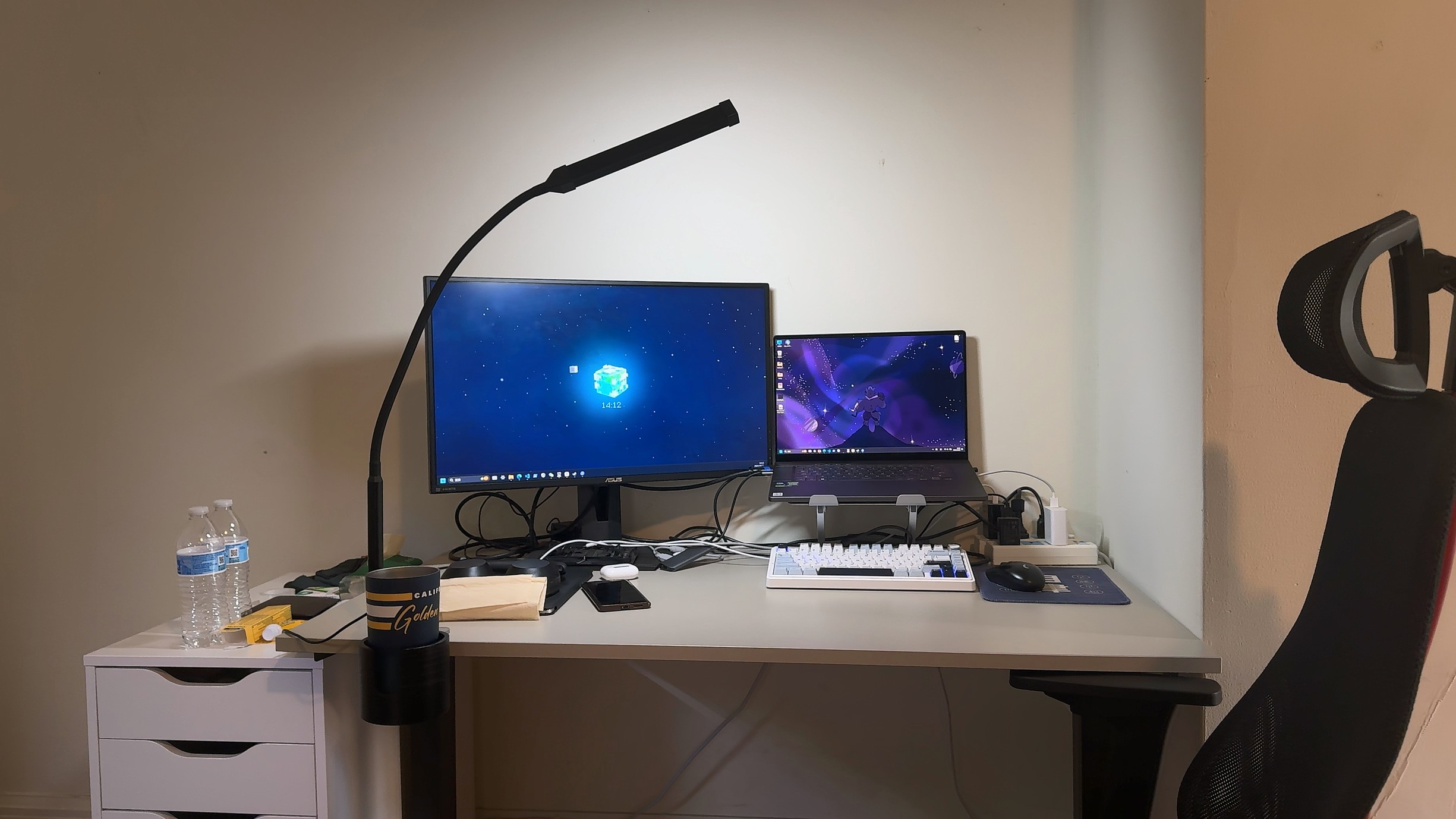
|
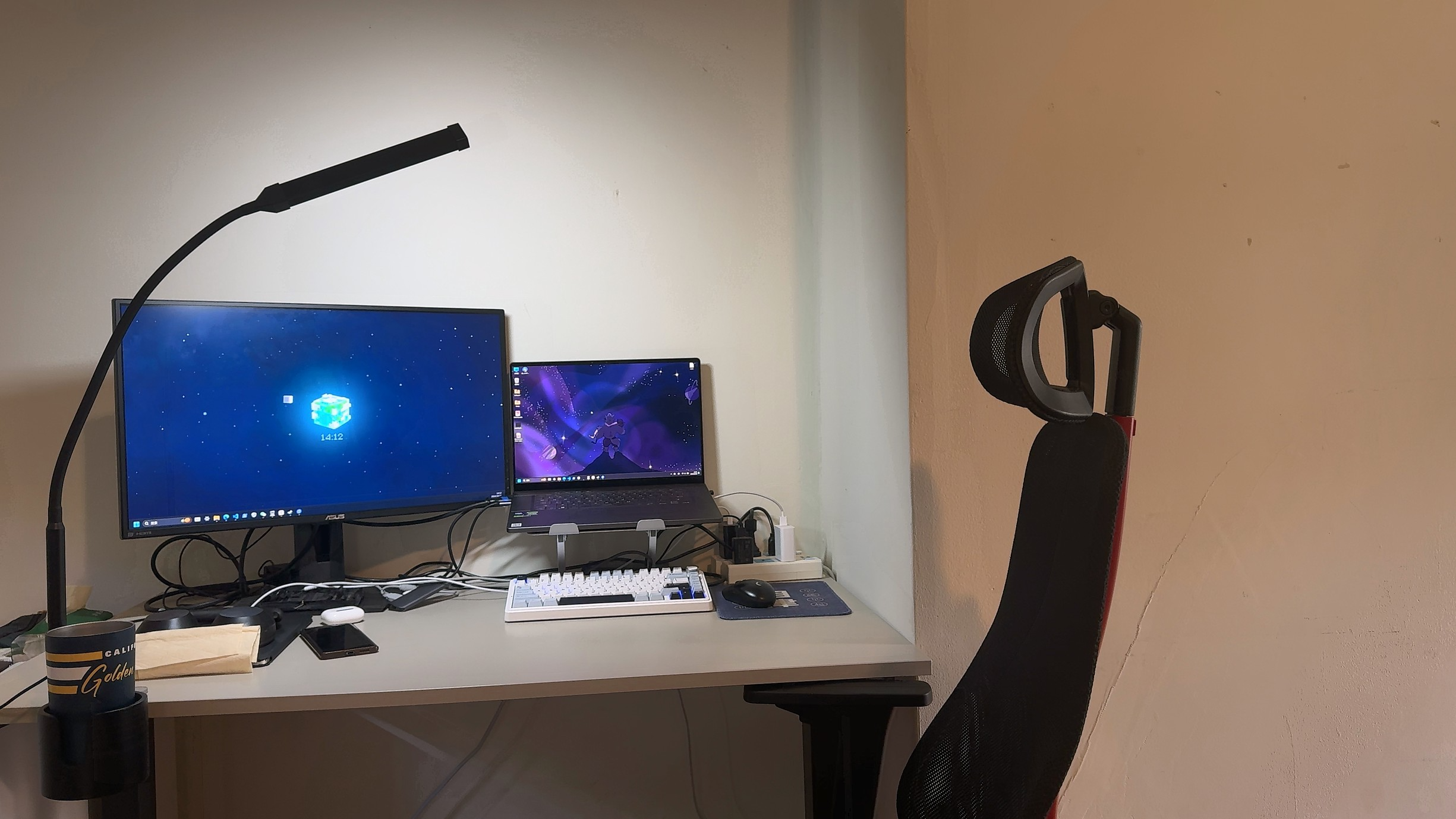
|
Project 4b: Automatic Image Panorama
Here we derive a method to detect corresponding points automatically.
Thus, the image panorama process will be completely automatic, without manually registering points.
Harris Corner Detector
We can implement Harris corner detector, a classic method to find corners in the image.
The basic idea of Harris corner detector is: slide a window on the image, and sense the change of pixel values.
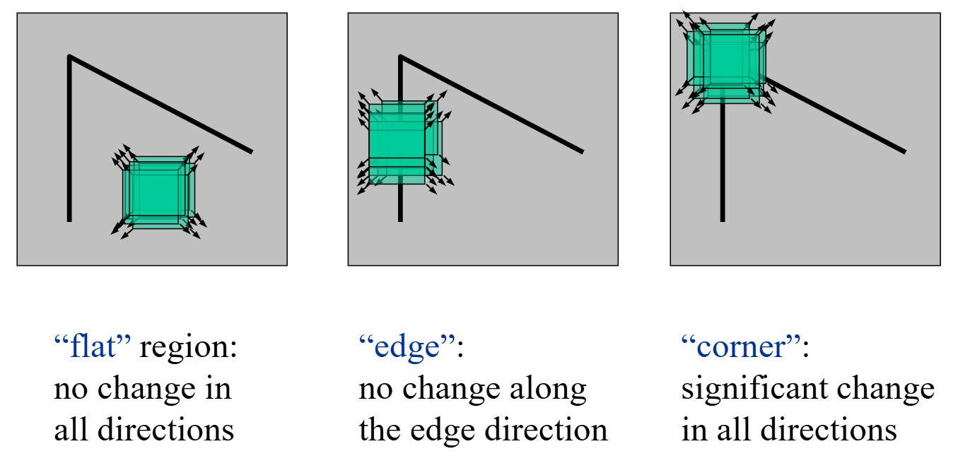
First, we define the change in appearance of window W for the shift \([u, v]\) as follows: \[ E(u, v) = \sum_{(x, y) \in W}{I(x + u, y + v) - I(x, y)} \]
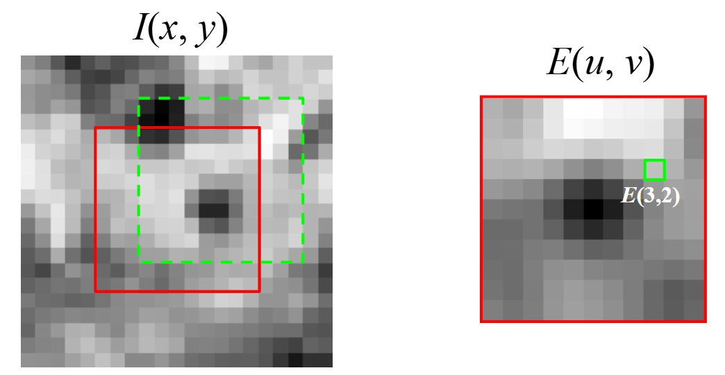
Then, we use a First-order Taylor approximation for small motions \([u, v]\): \[ \begin{aligned} I(x+u, y+v) &= I(x, y) + I_x u + I_y v + \text{higher order terms} \\ &\approx I(x, y) + I_x u + I_y v \\ &= I(x, y) + \begin{bmatrix} I_x & I_y \end{bmatrix} \begin{bmatrix} u \\ v \end{bmatrix} \end{aligned} \] Plugging this into \(E(u, v)\), we would get: \[ \begin{aligned} E(u, v) &= \sum_{(x, y) \in W} \left[I(x+u, y+v) - I(x, y)\right]^2 \\ &\approx \sum_{(x, y) \in W} \left[I(x, y) + \begin{bmatrix} I_x & I_y \end{bmatrix} \begin{bmatrix} u \\ v \end{bmatrix} - I(x, y)\right]^2 \\ &= \sum_{(x, y) \in W} \left(\begin{bmatrix} I_x & I_y \end{bmatrix} \begin{bmatrix} u \\ v \end{bmatrix}\right)^2 \\ &= \sum_{(x, y) \in W} \begin{bmatrix} u & v \end{bmatrix} \begin{bmatrix} I_x^2 & I_x I_y \\ I_x I_y & I_y^2 \end{bmatrix} \begin{bmatrix} u \\ v \end{bmatrix} \end{aligned} \]
This gives us the second moment matrix \(M\), which is a approximate of local change on images. \[ M = \begin{bmatrix} I_x^2 & I_x I_y \\ I_x I_y & I_y^2 \end{bmatrix} \]
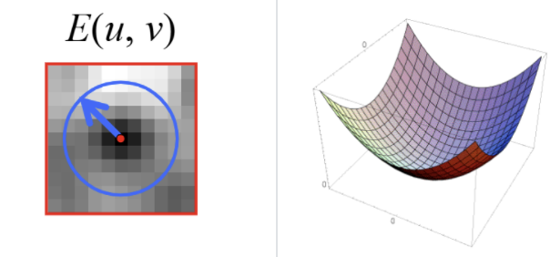
Therefore, we may use this quadratic form's eigenvalues and eigenvectors to describe a rotation-invariant corner strength.

Here, we calculate this function value as "corner strength": \[ R = \det(M) - k * \text{tr}(M)^2 \] where \(\det(M) = \lambda_1 * \lambda_2\), \(\text{tr}(M) = \lambda_1 + \lambda_2\).
Note that \(k\) is an empirical value, usually between \([0.04, 0.06]\). If this value is bigger, less corners are detected, and vice versa.
Summary:
- Compute Gaussian derivatives at each pixel
- Compute second moment matrix M in a Gaussian window around each pixel
- Compute corner response function R & Threshold R
Example Results:
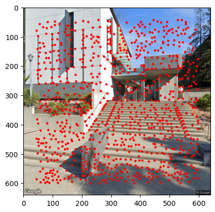
|
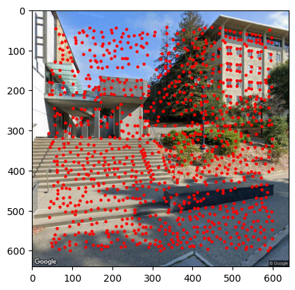
|

|
Adaptive Non-Maximal Suppression
Since the computational cost of matching is superlinear in the number of interest points, it is desirable to restrict the number of interest points extracted from each image. Also, we wish the interest points are spatially well-distributed. Hence, we implement ANMS (Adaptive Non-Maximal Suppression) to prune some points.
Method: Interest points are suppressed based on the corner strength \(R\), and only those that are a maximum in a neighborhood of radius \(r\) pixels are retained.
In practice we robustify the non-maximal suppression by requiring that a neighbor has a sufficiently larger strength. Thus the minimum suppression radius \(r_i\) is given by: \[ r_i = \min_{j} |x_i - x_j|, \text{s.t.} f(x_i) < c_{\text{robust}}f(x_j), X_J \in I \] where where \(x_i\) is a 2D interest point image location, and \(I\) is the set of all interest point location.
Note that \(c_j\) is an empirical value, usually taking \(0.9\).
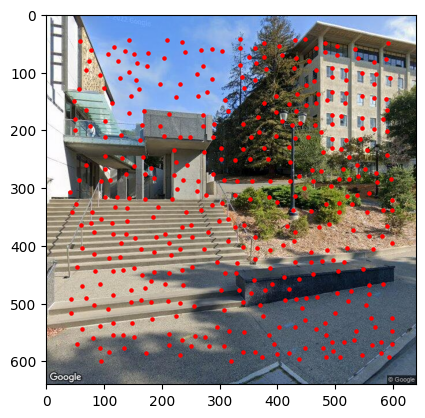
Example results:


Left: w/o pruning; Right: with ANMS pruning
Feature Descriptor Extraction
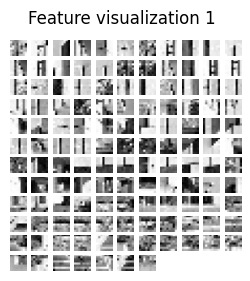
For each filtered interest point, we extract a feature descriptor for it. This is to facilitate our matching process, providing more information instead of a single pixel R value.
In this project, we simply extract a 8*8 axis-aligned box, down-sampled from a 40*40 box, centered by any interest point.
Here are some example results:
Feature Matching
Here, we implement an index to describe matching error, and then threshold on it to filter correctly matched points.
To be specific, the ratio of the closest to the second closest (1NN/2NN) is implemented.
This value is thresholded by an empirical value 0.67 according to the following graph.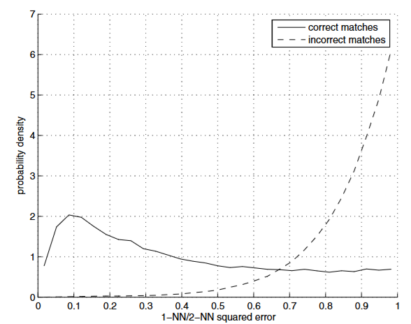
Here is an example after pruning points.
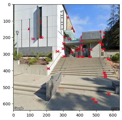

RANSAC Homography Estimation
As can be read from the image, there are still some outliers that are incorrectly matched. Hence we use RANSAC (RaNdom SAmple Consensus) to calculate a robust transform matrix.
RANSAC basically iterates a lot of times, each time choosing some points from the interest point list and calculate a homography matrix. Then, the algorithm checks if the points projected by the homography matrix are correct (meaning they are close to some other point in the plane that the image is projected to.)
Here is an example after calculating a robust transform matrix by RANSAC:
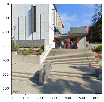
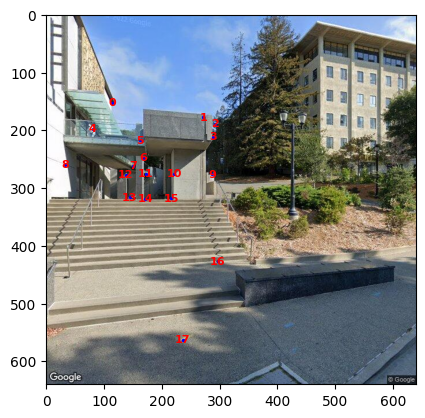
With the homography matrix, we can repeat the steps in project 4a to calculate a completely automatic image panorama!
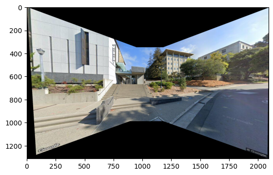
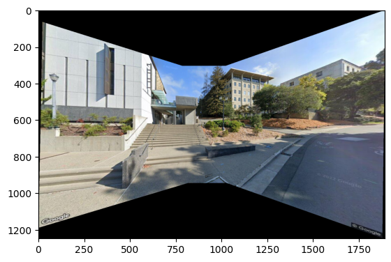
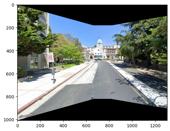
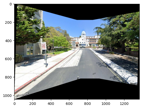
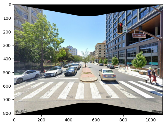
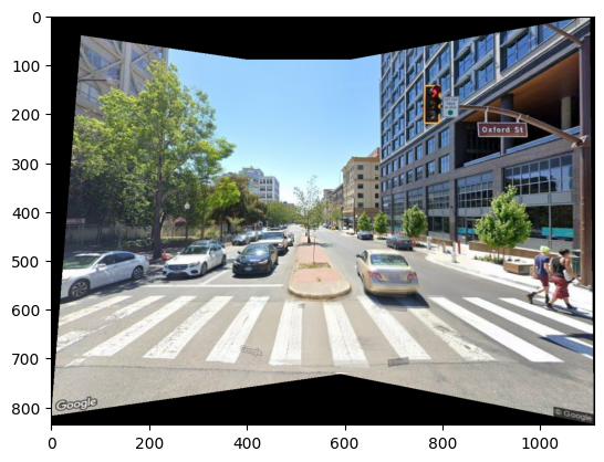
Result Comparison
|
|
|
|
|
|
Left: Automatic correspondence detection panorama; Right: Manual registering points panorama
Remark: Due to some errors in manually registering points, the last image in the right has been incorrect; but the automatic panorama's results are correct.
Project 4b: Result Gallery
Sather Gate
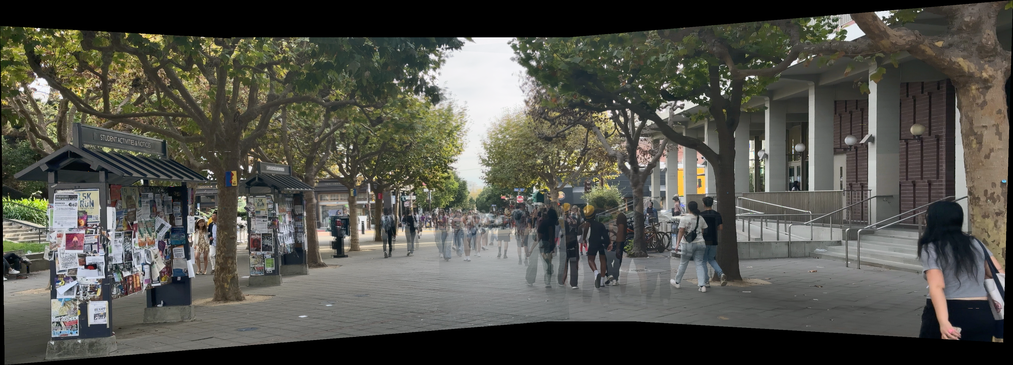
Somewhere near RSF
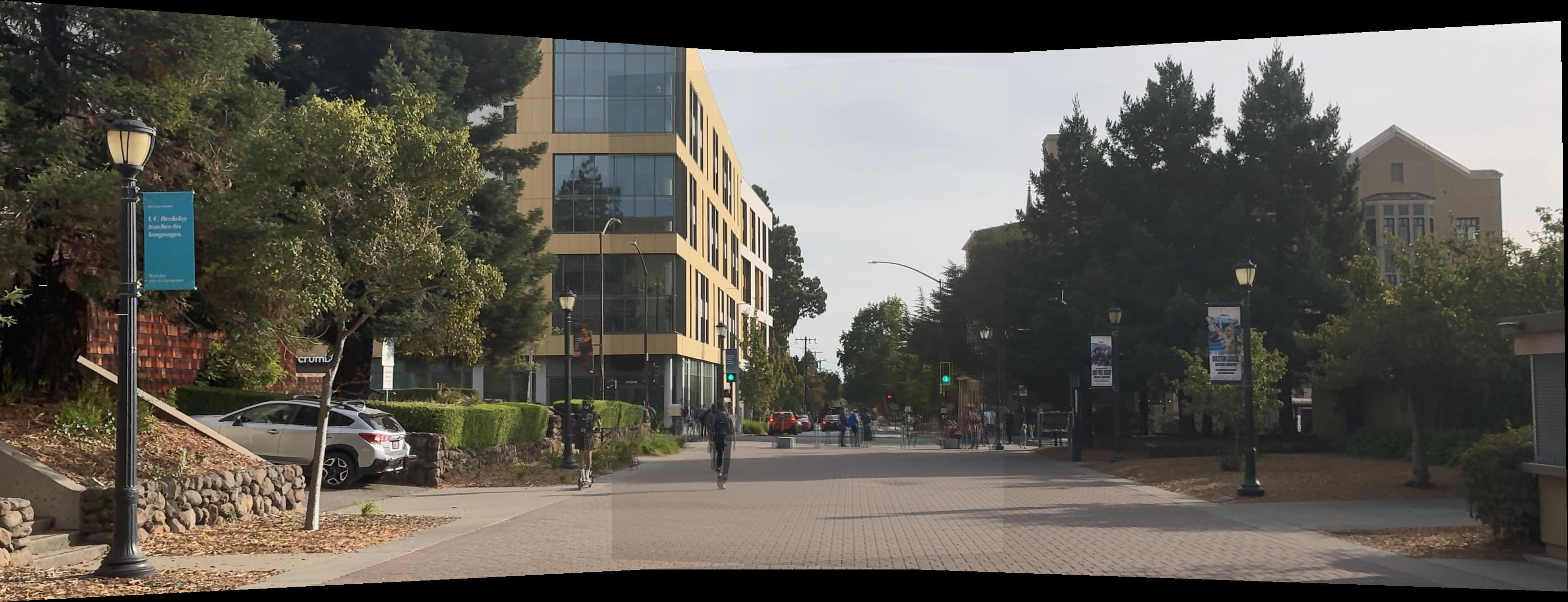
Lower plaza

Summaries and Takeaways
- From what HAS been implemented:
- Start from simple ideas. Corner detection is a hard job, but detecting the change in a small sliding window is not.
- Do it inversely. Direct projection makes it hard to grid points, but inverse-sampling makes it much simpler and parallelizable.
- From what has NOT been implemented:
- Make it multi-resolution. If you can'd detect corners in multiple scales, do it multiple times with different window sizes.
- Use transform-invariant descriptors. For example, eigenvalues. Or, make the corner descriptor box aligned to corner direction, instead of the axes.