UC-Berkeley 24FA CV Project 2:
Fun with Sobel, Gaussian Filters and Image Pyramids/Stacks; Blend Images by Band-Pass Filters.

Roadmap
This project involves three parts:
- Image Derivatives
- Image Filtering & Hybrid: A Reproduction of Paper (SIGGRAPH 2006)
- Multi-Resolution Blending: A Reproduction of Paper
Part I: Image Derivatives
Finite Difference Operators
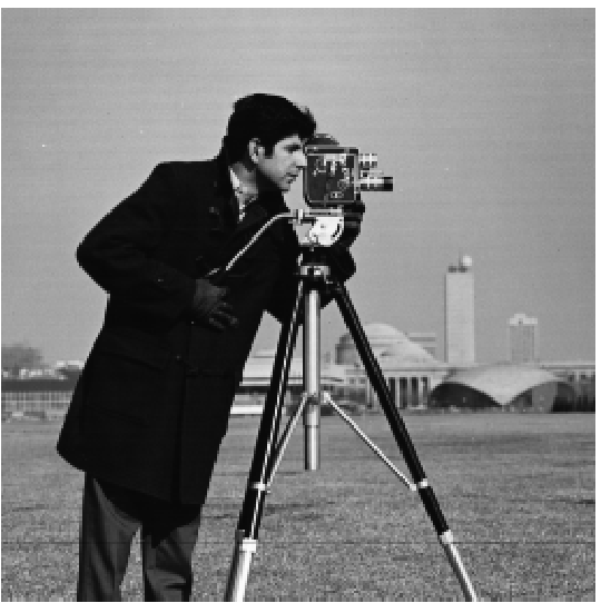
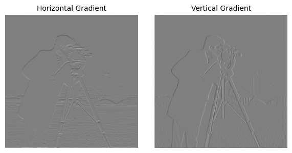
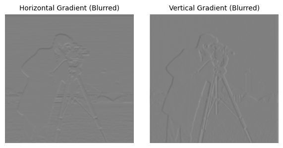
The simplest way to compute derivatives on images is by convolving the image with finite difference operators (FODs). Take \(D_x = \begin{bmatrix}1 & -1 \end{bmatrix}\) as an example, for each pixel in the resulting image (excepting those on the edge), they are equal to the original pixel minus its neighbor to the right. This operator is hence sensitive to vertical gradients.
Similarly, \(D_y = \begin{bmatrix}1 \\ -1 \end{bmatrix}\) is sensitive to horizontal gradients.
Here is an example of convolving the image with FOD operator:
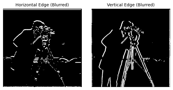
Furthermore, we can binarize the image. An appropriate threshold will filter all the edges from this gradient image.
Here is an example of binarizing the gradient image:
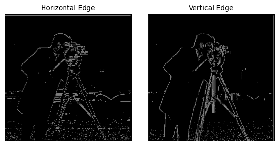
Details: Suppose pixel \(\in [0, 1]\).
The threshold is
np.logical_or(im > 0.57, im < 0.43)
Derivative of Gaussian Filter
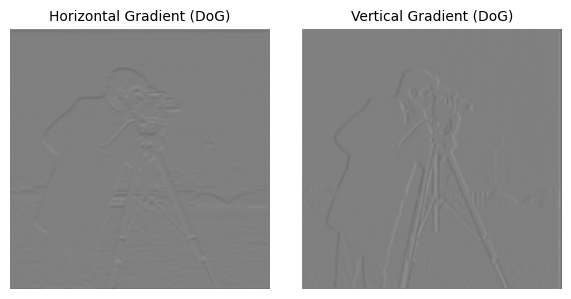
From the upper result, we notice that it's rather noisy. This is usually introduced by those high-frequency components in the image, which doesn't contribute to edges but literally causes a change in gradient. Hence, we introduce Gaussian Filters to get rid of those noises.
Here is an example of implementing Gaussian Filters before calculating image gradients:
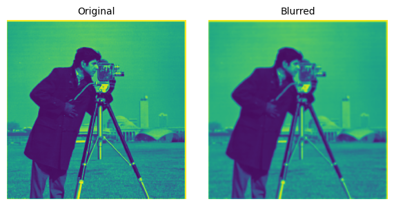
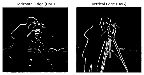
The threshold is:
np.logical_or(im > 0.52, im < 0.42)As the difference, implementing Gaussian filters can remove those sparkling noises in the picture. (Especially for the lawn, the effect is obvious). However, the tradeoff is that some edges are weakened. Take a look at those houses further away, their edges are simply omitted because there isn't a strong gradient at all.
Since convolution operation is commutative, i.e. \[ Img * Gaus * D_x = Img * (Gaus * D_x) \] we can introduce Derivative of Gaussian Filter, defined as \(Gaus * D_x\) or \(Gaus * D_y\). We can verify that convolving the image with Gaus & Dx is equivalent to convolving it with DoG filter.
Part II: Image Filtering
A Reproduction of Paper (SIGGRAPH 2006)
Image Sharpening
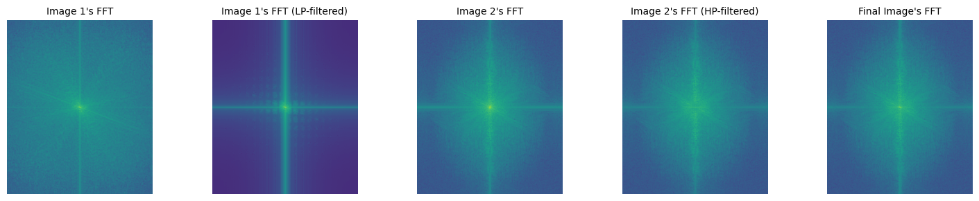
By Furrier Transform, we can observe that Gaussian Filter is essentially a Low-Pass Filter. Therefore, if we subtract the low-frequency component of an image from its original version, we can get those High-Frequency Components, which includes all edges, textures, etc.
We may blend these high frequency components with the original image itself by formula \(a * Image + (1-a) * HighFreq\). This will implement the process of Image Sharpening
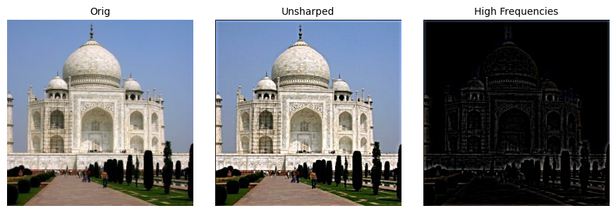
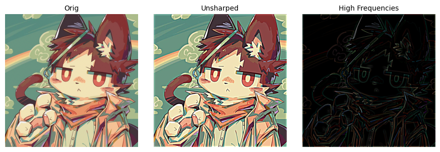
For evaluation, we will also blur the image first, and then sharpen it again to see what will happen. Here are some results:
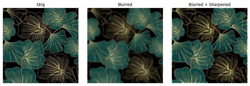
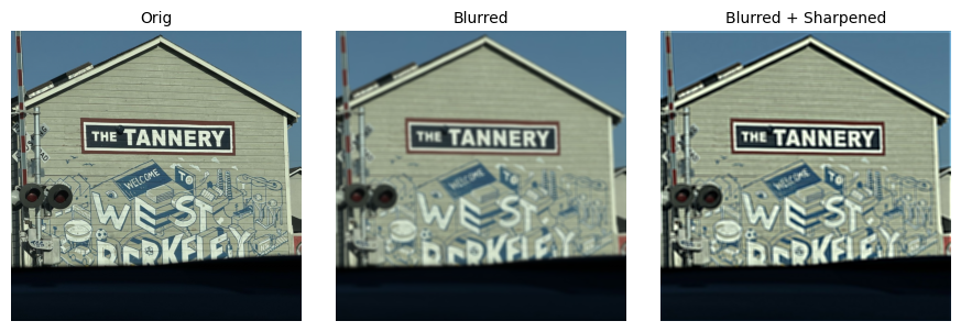
From the results, we may observe that sharpening may make the image look "sharper", but doesn't actually bring all the tiny textures back. Also, this may introduce reconstruction errors, where some lines seems thicker than their original version, which is introduced by gaussian filters.
This is because that the gaussian filters have already removed high-frequency components from the picture. If we re-sharpen it, we are actually enhancing the high-frequency components of the blurry image, which is not the high-frequency component of the original image. Hence error is introduced.
Hybrid Images
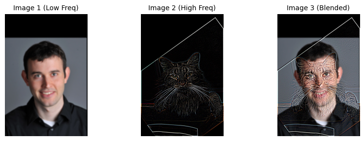
Here is a fun fact about frequency: High frequency of the signal may dominate perception when you are close to a image, but only low frequency of signal can be seen at a distance.
Hence, we may come up with some cool ideas: what about blending the high frequency of one signal with the low frequency of another signal, to get a image that look like A seeing from a distance but seems like B seeing closely?
From previous sections, we have already known how to extract the high/low frequency components from a image. Hence, lets blend them together!
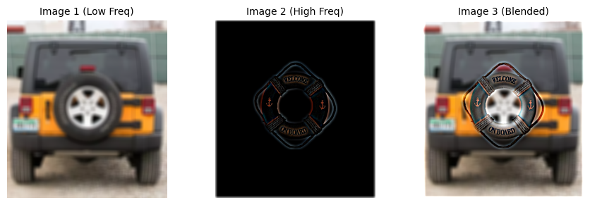
Here are some results:
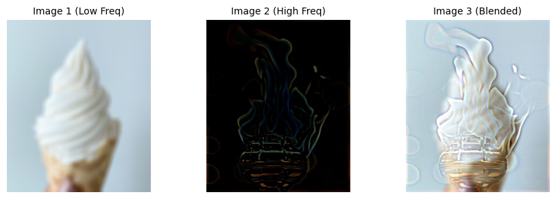
More Results
Failure Result Example
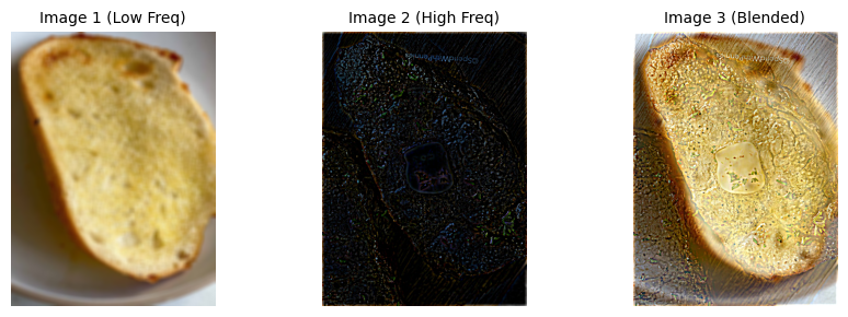
Explanation: It's a "perceptual" failure. In our cognition, the surface texture of the bread is not like a steak's, while the steak's color isn't yellow as well. Hence they don't "blend" together very well. Also, the HP Filter is not good at extracting the tiny textures on the steak. This also contributed to failure.
Part III: Multi-Resolution Blending
A Reproduction of Paper
Intuitive: if we simply implement alpha-blending on images, the results will look strange with unnatural transitions. How can we come up with a method to blend them together better?
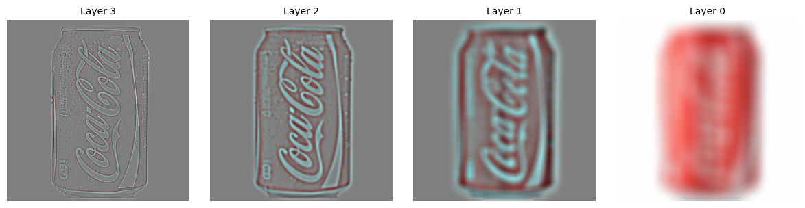
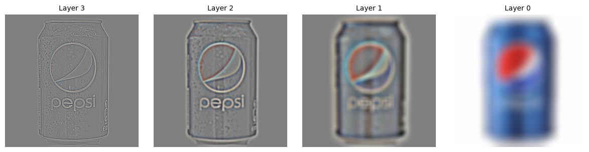
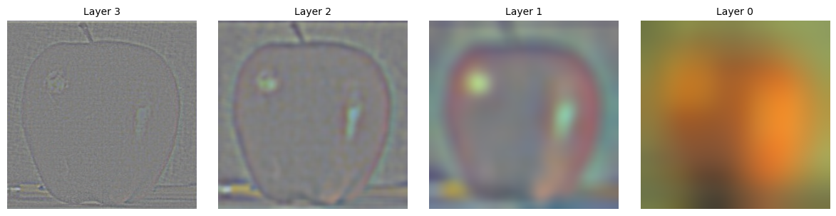
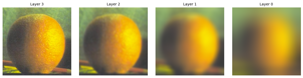
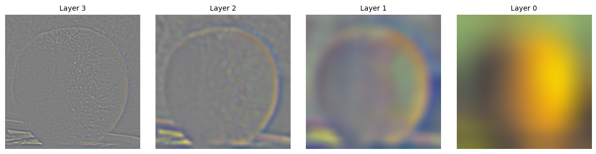
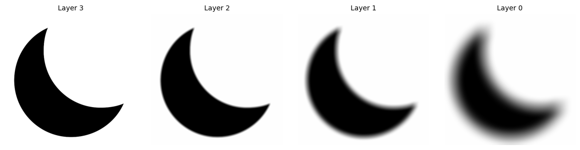
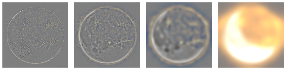
Gaussian and Laplacian Stacks
First, we introduce the Gaussian and Laplacian stack. This is to represent the image's different frequency components in a hierarchal way. For each level of image, we blur it and push it into stack.
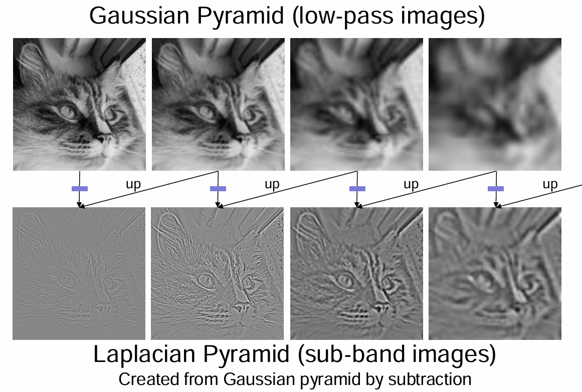
Image cited from CS180 FA24, UC Berkeley, Alexei Efros.
Multi-Resolution Blending
Here are some results (Gaussian Stacks & Laplacian Stacks):
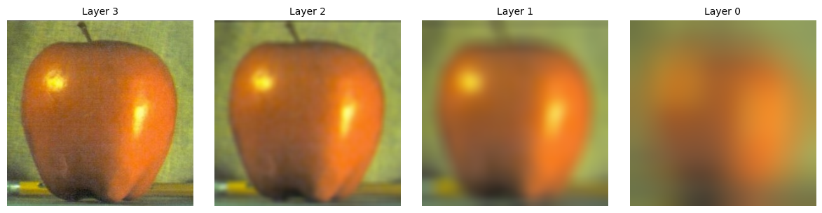
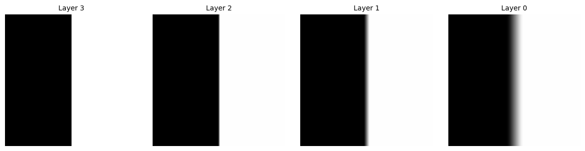
Also, for the convenience of blending, we also implement a Gaussian Stack on a mask.
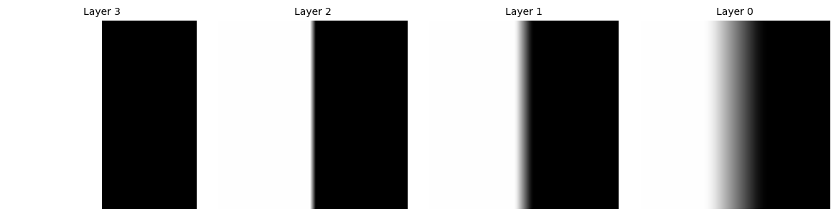
Everything has been prepared! We may simply blend images together, according to the mask value.
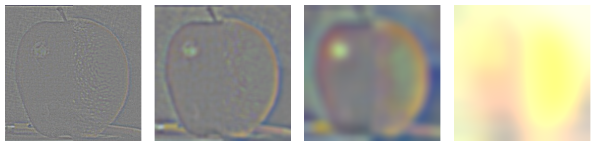
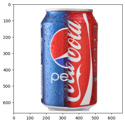
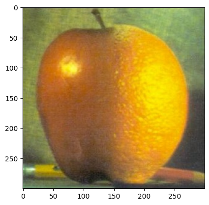
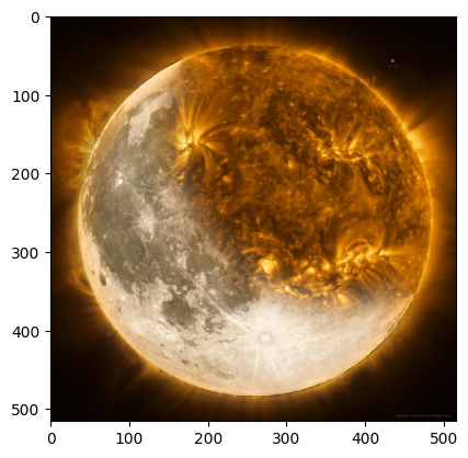
And here comes the juicy ora-pple! (Need to collapse the Laplacian Stack by adding all layers together)
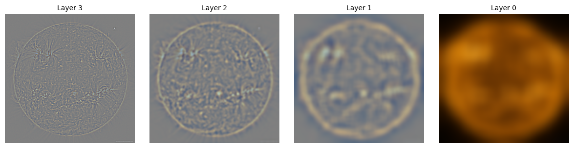
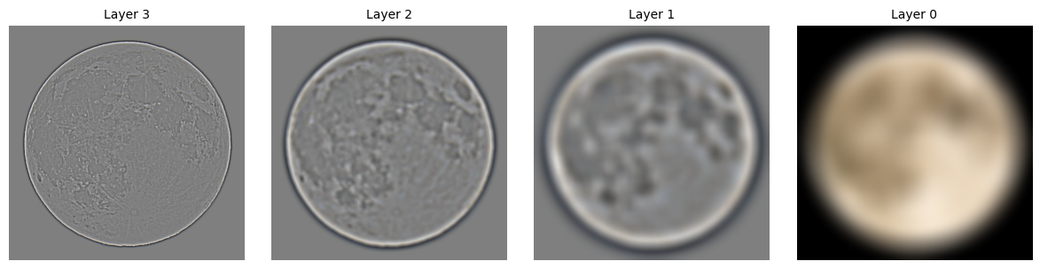
Here are some of more results:
Sun-Moon:
Coca-Pepsi: